Rolling Window Transformation

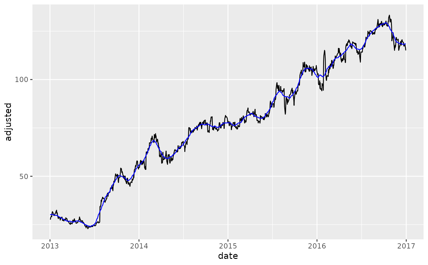
slidify_vec() applies a summary function to a rolling sequence of windows.

Usage

slidify_vec(
  .x,
  .f,
  ...,
  .period = 1,
  .align = c("center", "left", "right"),
  .partial = FALSE
)

Arguments

.x

A vector to have a rolling window transformation applied.

.f

A summary [function / formula]

• If a function, e.g. mean, the function is used with any additional arguments, ....

• If a formula, e.g. ~ mean(., na.rm = TRUE), it is converted to a function.

This syntax allows you to create very compact anonymous functions.

...

Additional arguments passed on to the .f function.

.period

The number of periods to include in the local rolling window. This is effectively the "window size".

.align

One of "center", "left" or "right".

.partial

Should the moving window be allowed to return partial (incomplete) windows instead of NA values. Set to FALSE by default, but can be switched to TRUE to remove NA's.

Value

A numeric vector

Details

The slidify_vec() function is a wrapper for slider::slide_vec() with parameters simplified "center", "left", "right" alignment.

Vector Length In == Vector Length Out

NA values or .partial values are always returned to ensure the length of the return vector is the same length of the incoming vector. This ensures easier use with dplyr::mutate().

Alignment

Rolling functions generate .period - 1 fewer values than the incoming vector. Thus, the vector needs to be aligned. Alignment of the vector follows 3 types:

• Center: NA or .partial values are divided and added to the beginning and end of the series to "Center" the moving average. This is common for de-noising operations. See also [smooth_vec()] for LOESS without NA values.

• Left: NA or .partial values are added to the end to shift the series to the Left.

• Right: NA or .partial values are added to the beginning to shif the series to the Right. This is common in Financial Applications such as moving average cross-overs.

Partial Values

• The advantage to using .partial values vs NA padding is that the series can be filled (good for time-series de-noising operations).

• The downside to partial values is that the partials can become less stable at the regions where incomplete windows are used.

If instability is not desirable for de-noising operations, a suitable alternative is smooth_vec(), which implements local polynomial regression.

References

• Slider R Package by Davis Vaughan

See also

Modeling and More Complex Rolling Operations:

• step_slidify() - Roll apply for tidymodels modeling

• tk_augment_slidify() - Add many rolling columns group-wise

• slidify() - Turn any function into a rolling function. Great for rolling cor, rolling regression, etc.

• For more complex rolling operations, check out the slider R package.

Vectorized Transformation Functions:

• Box Cox Transformation: box_cox_vec()

• Lag Transformation: lag_vec()

• Differencing Transformation: diff_vec()

• Rolling Window Transformation: slidify_vec()

• Loess Smoothing Transformation: smooth_vec()

• Fourier Series: fourier_vec()

• Missing Value Imputation for Time Series: ts_impute_vec()

Examples

library(dplyr)
library(ggplot2)

# Training Data
FB_tbl <- FANG %>%
    filter(symbol == "FB") %>%
    select(symbol, date, adjusted)

# ---- FUNCTION FORMAT ----
# - The `.f = mean` function is used. Argument `na.rm = TRUE` is passed as ...
FB_tbl %>%
    mutate(adjusted_30_ma = slidify_vec(
        .x      = adjusted,
        .period = 30,
        .f      = mean,
        na.rm   = TRUE,
        .align  = "center")) %>%
        ggplot(aes(date, adjusted)) +
        geom_line() +
        geom_line(aes(y = adjusted_30_ma), color = "blue", na.rm = TRUE)


# ---- FORMULA FORMAT ----
# - Anonymous function `.f = ~ mean(., na.rm = TRUE)` is used
FB_tbl %>%
    mutate(adjusted_30_ma = slidify_vec(
        .x      = adjusted,
        .period = 30,
        .f      = ~ mean(., na.rm = TRUE),
        .align  = "center")) %>%
        ggplot(aes(date, adjusted)) +
        geom_line() +
        geom_line(aes(y = adjusted_30_ma), color = "blue", na.rm = TRUE)


# ---- PARTIAL VALUES ----
# - set `.partial = TRUE`
FB_tbl %>%
    mutate(adjusted_30_ma = slidify_vec(
        .x       = adjusted,
        .f       = ~ mean(., na.rm = TRUE),
        .period  = 30,
        .align   = "center",
        .partial = TRUE)) %>%
        ggplot(aes(date, adjusted)) +
        geom_line() +
        geom_line(aes(y = adjusted_30_ma), color = "blue")


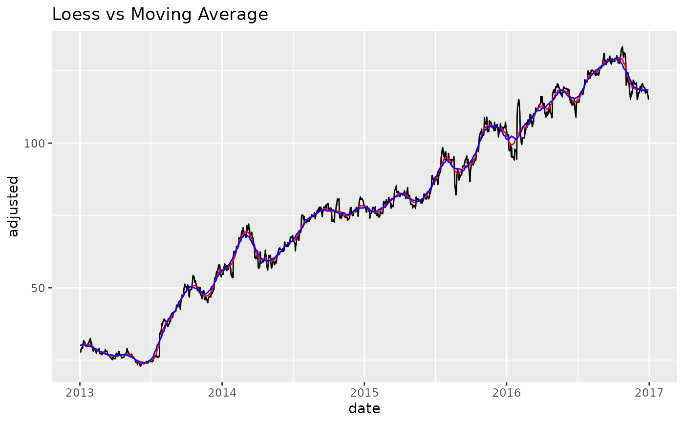
# ---- Loess vs Moving Average ----
# - Loess: Using `.degree = 0` to make less flexible. Comparable to a moving average.

FB_tbl %>%
    mutate(
        adjusted_loess_30 = smooth_vec(adjusted, period = 30, degree = 0),
        adjusted_ma_30    = slidify_vec(adjusted, .f = mean,
                                           .period = 30, .partial = TRUE)
    ) %>%
    ggplot(aes(date, adjusted)) +
    geom_line() +
    geom_line(aes(y = adjusted_loess_30), color = "red") +
    geom_line(aes(y = adjusted_ma_30), color = "blue") +
    labs(title = "Loess vs Moving Average")