Smoothing Transformation using Loess

smooth_vec() applies a LOESS transformation to a numeric vector.

Usage

smooth_vec(x, period = 30, span = NULL, degree = 2)

Arguments

x

A numeric vector to have a smoothing transformation applied.

period

The number of periods to include in the local smoothing. Similar to window size for a moving average. See details for an explanation period vs span specification.

span

The span is a percentage of data to be included in the smoothing window. Period is preferred for shorter windows to fix the window size. See details for an explanation period vs span specification.

degree

The degree of the polynomials to be used. Accetable values (least to most flexible): 0, 1, 2. Set to 2 by default for 2nd order polynomial (most flexible).

Value

A numeric vector

Details

Benefits:

• When using period, the effect is similar to a moving average without creating missing values.

• When using span, the effect is to detect the trend in a series using a percentage of the total number of observations.

Loess Smoother Algorithm This function is a simplified wrapper for the stats::loess() with a modification to set a fixed period rather than a percentage of data points via a span.

Why Period vs Span? The period is fixed whereas the span changes as the number of observations change.

When to use Period? The effect of using a period is similar to a Moving Average where the Window Size is the Fixed Period. This helps when you are trying to smooth local trends. If you want a 30-day moving average, specify period = 30.

When to use Span? Span is easier to specify when you want a Long-Term Trendline where the window size is unknown. You can specify span = 0.75 to locally regress using a window of 75% of the data.

See also

Loess Modeling Functions:

• step_smooth() - Recipe for tidymodels workflow

Additional Vector Functions:

• Box Cox Transformation: box_cox_vec()

• Lag Transformation: lag_vec()

• Differencing Transformation: diff_vec()

• Rolling Window Transformation: slidify_vec()

• Loess Smoothing Transformation: smooth_vec()

• Fourier Series: fourier_vec()

• Missing Value Imputation for Time Series: ts_impute_vec()

Examples

library(dplyr)
library(ggplot2)

# Training Data
FB_tbl <- FANG %>%
    filter(symbol == "FB") %>%
    select(symbol, date, adjusted)

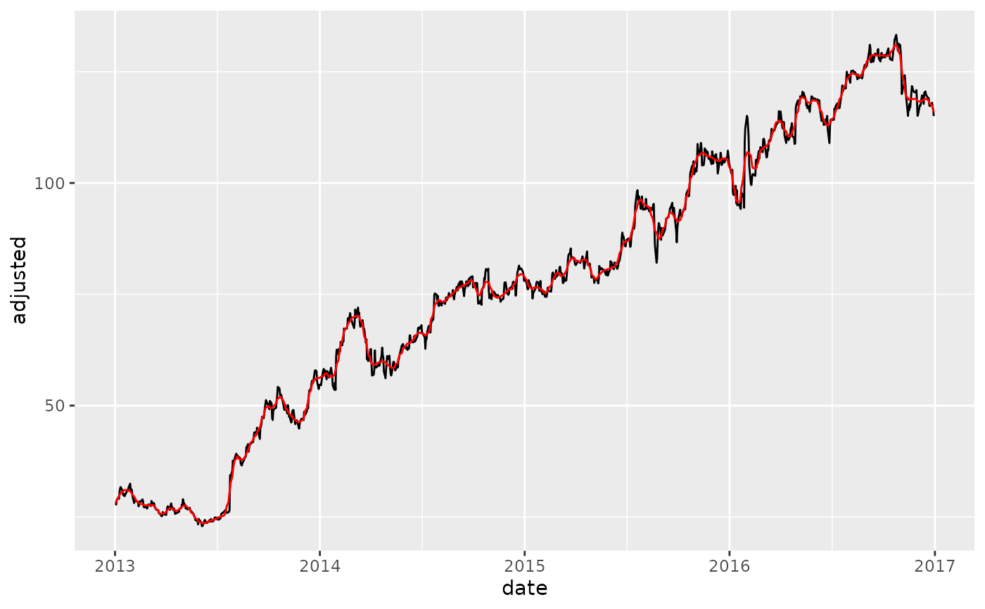
# ---- PERIOD ----

FB_tbl %>%
    mutate(adjusted_30 = smooth_vec(adjusted, period = 30, degree = 2)) %>%
    ggplot(aes(date, adjusted)) +
    geom_line() +
    geom_line(aes(y = adjusted_30), color = "red")


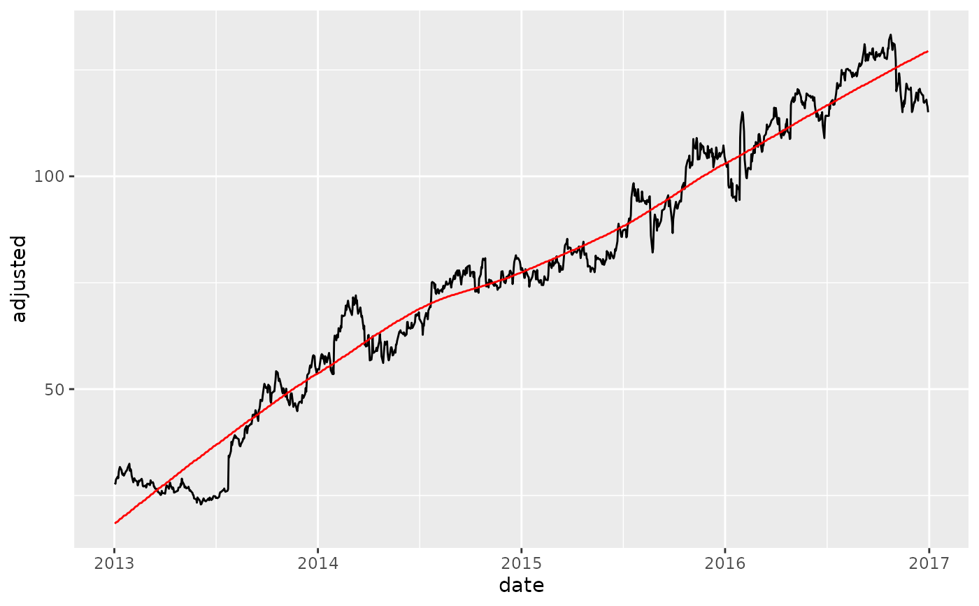
# ---- SPAN ----

FB_tbl %>%
    mutate(adjusted_30 = smooth_vec(adjusted, span = 0.75, degree = 2)) %>%
    ggplot(aes(date, adjusted)) +
    geom_line() +
    geom_line(aes(y = adjusted_30), color = "red")


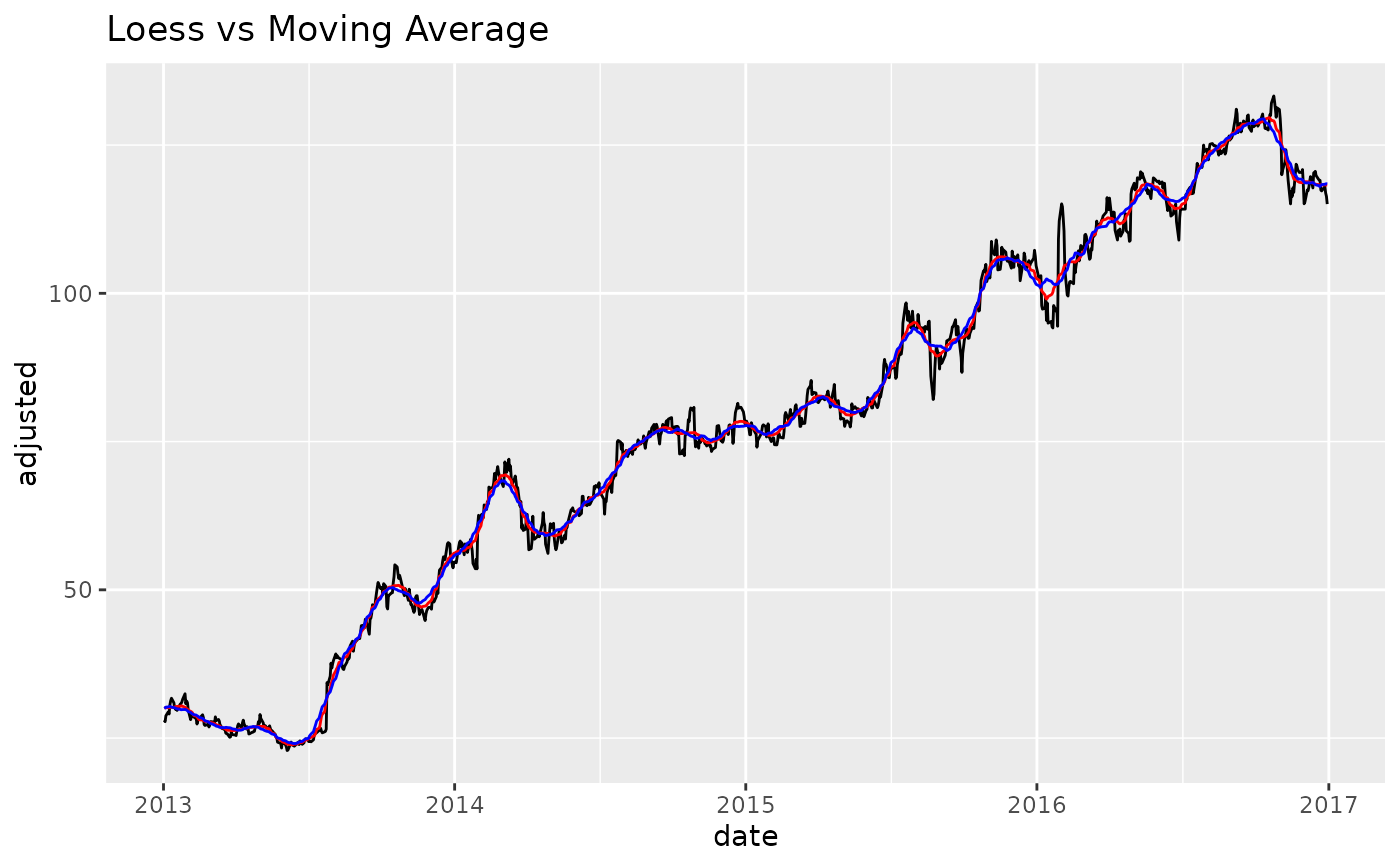
# ---- Loess vs Moving Average ----
# - Loess: Using `degree = 0` to make less flexible. Comperable to a moving average.

FB_tbl %>%
    mutate(
        adjusted_loess_30 = smooth_vec(adjusted, period = 30, degree = 0),
        adjusted_ma_30    = slidify_vec(adjusted, .period = 30,
                                        .f = mean, .partial = TRUE)
    ) %>%
    ggplot(aes(date, adjusted)) +
    geom_line() +
    geom_line(aes(y = adjusted_loess_30), color = "red") +
    geom_line(aes(y = adjusted_ma_30), color = "blue") +
    labs(title = "Loess vs Moving Average")