Anomaly Detection

Anomaly detection is an important part of time series analysis:

Detecting anomalies can signify special events
Cleaning anomalies can improve forecast error

This tutorial will cover:

library(dplyr)
library(purrr)
library(timetk)

Data

This tutorial will use the wikipedia_traffic_daily dataset:

wikipedia_traffic_daily %>% glimpse()

## Rows: 5,500
## Columns: 3
## $ Page  <chr> "Death_of_Freddie_Gray_en.wikipedia.org_mobile-web_all-agents", …
## $ date  <date> 2015-07-01, 2015-07-02, 2015-07-03, 2015-07-04, 2015-07-05, 201…
## $ value <dbl> 791, 704, 903, 732, 558, 504, 543, 1156, 1196, 701, 829, 838, 11…

Visualization

Using the plot_time_series() function, we can interactively detect anomalies at scale.

wikipedia_traffic_daily %>%
  group_by(Page) %>%
  plot_time_series(date, value, .facet_ncol = 2)

Anomalize: breakdown, identify, and clean in 1 easy step

The anomalize() function is a feature rich tool for performing anomaly detection. Anomalize is group-aware, so we can use this as part of a normal pandas groupby chain. In one easy step:

We breakdown (decompose) the time series
Analyze it’s remainder (residuals) for spikes (anomalies)
Clean the anomalies if desired

anomalize_tbl <- wikipedia_traffic_daily %>%
  group_by(Page) %>%
  anomalize(
      .date_var      = date, 
      .value         = value,
      .iqr_alpha     = 0.05,
      .max_anomalies = 0.20,
      .message       = FALSE
  )

anomalize_tbl %>% glimpse()

## Rows: 5,500
## Columns: 13
## Groups: Page [10]
## $ Page              <chr> "Death_of_Freddie_Gray_en.wikipedia.org_mobile-web_a…
## $ date              <date> 2015-07-01, 2015-07-02, 2015-07-03, 2015-07-04, 201…
## $ observed          <dbl> 791, 704, 903, 732, 558, 504, 543, 1156, 1196, 701, …
## $ season            <dbl> 9.2554027, 13.1448419, -20.5421912, -24.0966839, 0.4…
## $ trend             <dbl> 748.1907, 744.3101, 740.4296, 736.5490, 732.6684, 72…
## $ remainder         <dbl> 33.553930, -53.454953, 183.112637, 19.547687, -175.1…
## $ seasadj           <dbl> 781.7446, 690.8552, 923.5422, 756.0967, 557.5091, 50…
## $ anomaly           <chr> "No", "No", "No", "No", "No", "No", "No", "No", "No"…
## $ anomaly_direction <dbl> 0, 0, 0, 0, 0, 0, 0, 0, 0, 0, 0, 0, 0, 0, 0, 0, 0, 0…
## $ anomaly_score     <dbl> 83.50187, 170.51076, 66.05683, 97.50812, 292.21517, …
## $ recomposed_l1     <dbl> -328.3498, -328.3409, -365.9085, -373.3435, -352.636…
## $ recomposed_l2     <dbl> 2077.354, 2077.362, 2039.795, 2032.360, 2053.067, 20…
## $ observed_clean    <dbl> 791.000, 704.000, 903.000, 732.000, 558.000, 504.000…

The anomalize() function returns:

The original grouping and datetime columns.
The seasonal decomposition: observed, seasonal, seasadj, trend, and remainder. The objective is to remove trend and seasonality such that the remainder is stationary and representative of normal variation and anomalous variations.
Anomaly identification and scoring: anomaly, anomaly_score, anomaly_direction. These identify the anomaly decision (Yes/No), score the anomaly as a distance from the centerline, and label the direction (-1 (down), zero (not anomalous), +1 (up)).
Recomposition: recomposed_l1 and recomposed_l2. Think of these as the lower and upper bands. Any observed data that is below l1 or above l2 is anomalous.
Cleaned data: observed_clean. Cleaned data is automatically provided, which has the outliers replaced with data that is within the recomposed l1/l2 boundaries. With that said, you should always first seek to understand why data is being considered anomalous before simply removing outliers and using the cleaned data.

The most important aspect is that this data is ready to be visualized, inspected, and modifications can then be made to address any tweaks you would like to make.

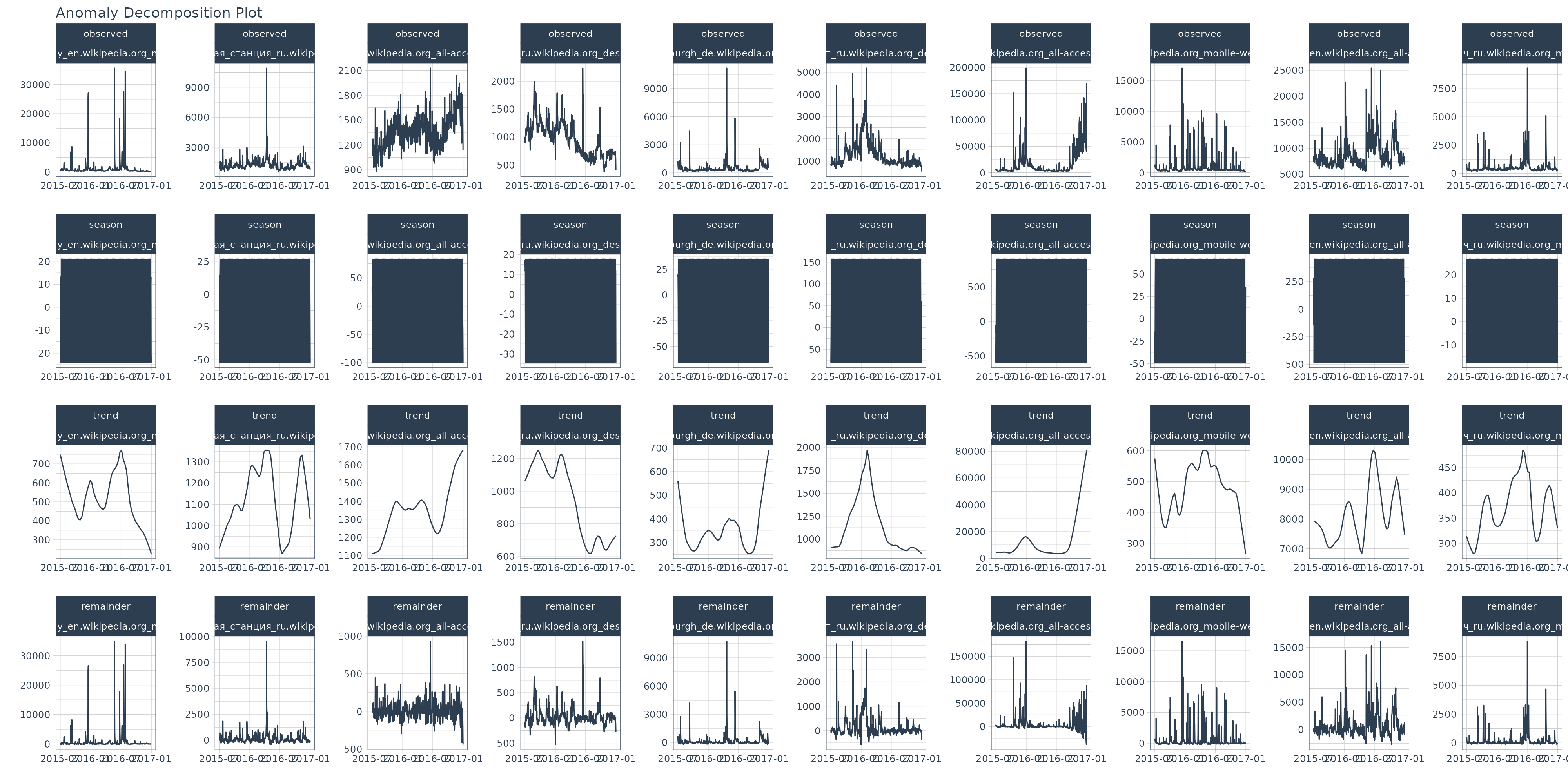
Anomaly Visualization 1: Seasonal Decomposition Plot

The first step in my normal process is to analyze the seasonal decomposition. I want to see what the remainders look like, and make sure that the trend and seasonality are being removed such that the remainder is centered around zero.

anomalize_tbl %>%
    group_by(Page) %>%
    plot_anomalies_decomp(
        .date_var = date, 
        .interactive = FALSE
    )

Anomaly Visualization 2: Anomaly Detection Plot

Once I’m satisfied with the remainders, my next step is to visualize the anomalies. Here I’m looking to see if I need to grow or shrink the remainder l1 and l2 bands, which classify anomalies.

anomalize_tbl %>%
    group_by(Page) %>%
    plot_anomalies(
        date,
        .facet_ncol = 2
    )

Anomaly Visualization 3: Anomalies Cleaned Plot

There are pros and cons to cleaning anomalies. I’ll leave that discussion for another time. But, should you be interested in seeing what your data looks like cleaned (with outliers removed), this plot will help you compare before and after.

anomalize_tbl %>%
    group_by(Page) %>%
    plot_anomalies_cleaned(
        date,
        .facet_ncol = 2
    )

Learning More

My Talk on High-Performance Time Series Forecasting

Time series is changing. Businesses now need 10,000+ time series forecasts every day. This is what I call a High-Performance Time Series Forecasting System (HPTSF) - Accurate, Robust, and Scalable Forecasting.

High-Performance Forecasting Systems will save companies MILLIONS of dollars. Imagine what will happen to your career if you can provide your organization a “High-Performance Time Series Forecasting System” (HPTSF System).

I teach how to build a HPTFS System in my High-Performance Time Series Forecasting Course. If interested in learning Scalable High-Performance Forecasting Strategies then take my course. You will learn:

Time Series Machine Learning (cutting-edge) with Modeltime - 30+ Models (Prophet, ARIMA, XGBoost, Random Forest, & many more)
NEW - Deep Learning with GluonTS (Competition Winners)
Time Series Preprocessing, Noise Reduction, & Anomaly Detection
Feature engineering using lagged variables & external regressors
Hyperparameter Tuning
Time series cross-validation
Ensembling Multiple Machine Learning & Univariate Modeling Techniques (Competition Winner)
Scalable Forecasting - Forecast 1000+ time series in parallel
and more.

Unlock the High-Performance Time Series Forecasting Course

Matt Dancho