Time Series Machine Learning

This vignette covers Machine Learning for Forecasting using the time-series signature, a collection calendar features derived from the timestamps in the time series.

Introduction

The time series signature is a collection of useful features that describe the time series index of a time-based data set. It contains a wealth of features that can be used to forecast time series that contain patterns.

In this vignette, the user will learn methods to implement machine learning to predict future outcomes in a time-based data set. The vignette example uses a well known time series dataset, the Bike Sharing Dataset, from the UCI Machine Learning Repository. The vignette follows an example where we’ll use timetk to build a basic Machine Learning model to predict future values using the time series signature. The objective is to build a model and predict the next six months of Bike Sharing daily counts.

Prerequisites

Before we get started, load the following packages.

library(dplyr)
library(timetk)
library(recipes)
library(parsnip)
library(workflows)
library(rsample)
# Used to convert plots from interactive to static
interactive = FALSE

Data

We’ll be using the Bike Sharing Dataset from the UCI Machine Learning Repository.

Source: Fanaee-T, Hadi, and Gama, Joao, ‘Event labeling combining ensemble detectors and background knowledge’, Progress in Artificial Intelligence (2013): pp. 1-15, Springer Berlin Heidelberg

# Read data
bike_transactions_tbl <- bike_sharing_daily %>%
  select(date = dteday, value = cnt)

bike_transactions_tbl

## # A tibble: 731 × 2
##    date       value
##    <date>     <dbl>
##  1 2011-01-01   985
##  2 2011-01-02   801
##  3 2011-01-03  1349
##  4 2011-01-04  1562
##  5 2011-01-05  1600
##  6 2011-01-06  1606
##  7 2011-01-07  1510
##  8 2011-01-08   959
##  9 2011-01-09   822
## 10 2011-01-10  1321
## # ℹ 721 more rows

Next, visualize the dataset with the plot_time_series() function. Toggle .interactive = TRUE to get a plotly interactive plot. FALSE returns a ggplot2 static plot.

bike_transactions_tbl %>%
  plot_time_series(date, value, .interactive = interactive)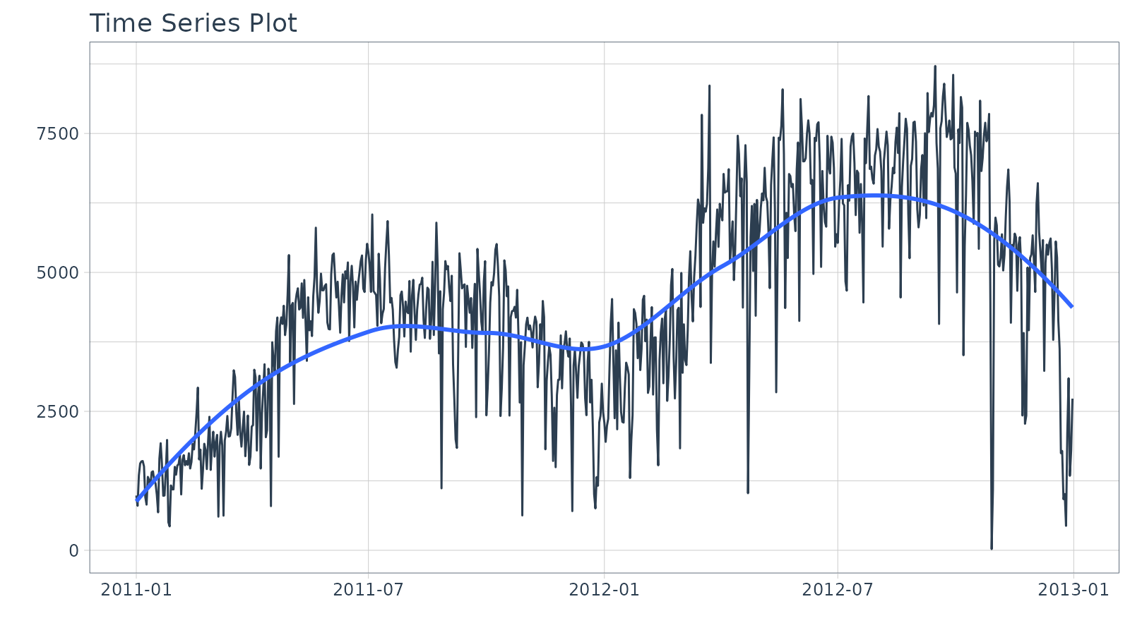

Train / Test

Next, use time_series_split() to make a train/test set.

Setting assess = "3 months" tells the function to use the last 3-months of data as the testing set.
Setting cumulative = TRUE tells the sampling to use all of the prior data as the training set.

splits <- bike_transactions_tbl %>%
  time_series_split(assess = "3 months", cumulative = TRUE)

Next, visualize the train/test split.

tk_time_series_cv_plan(): Converts the splits object to a data frame
plot_time_series_cv_plan(): Plots the time series sampling data using the “date” and “value” columns.

splits %>%
  tk_time_series_cv_plan() %>%
  plot_time_series_cv_plan(date, value, .interactive = interactive)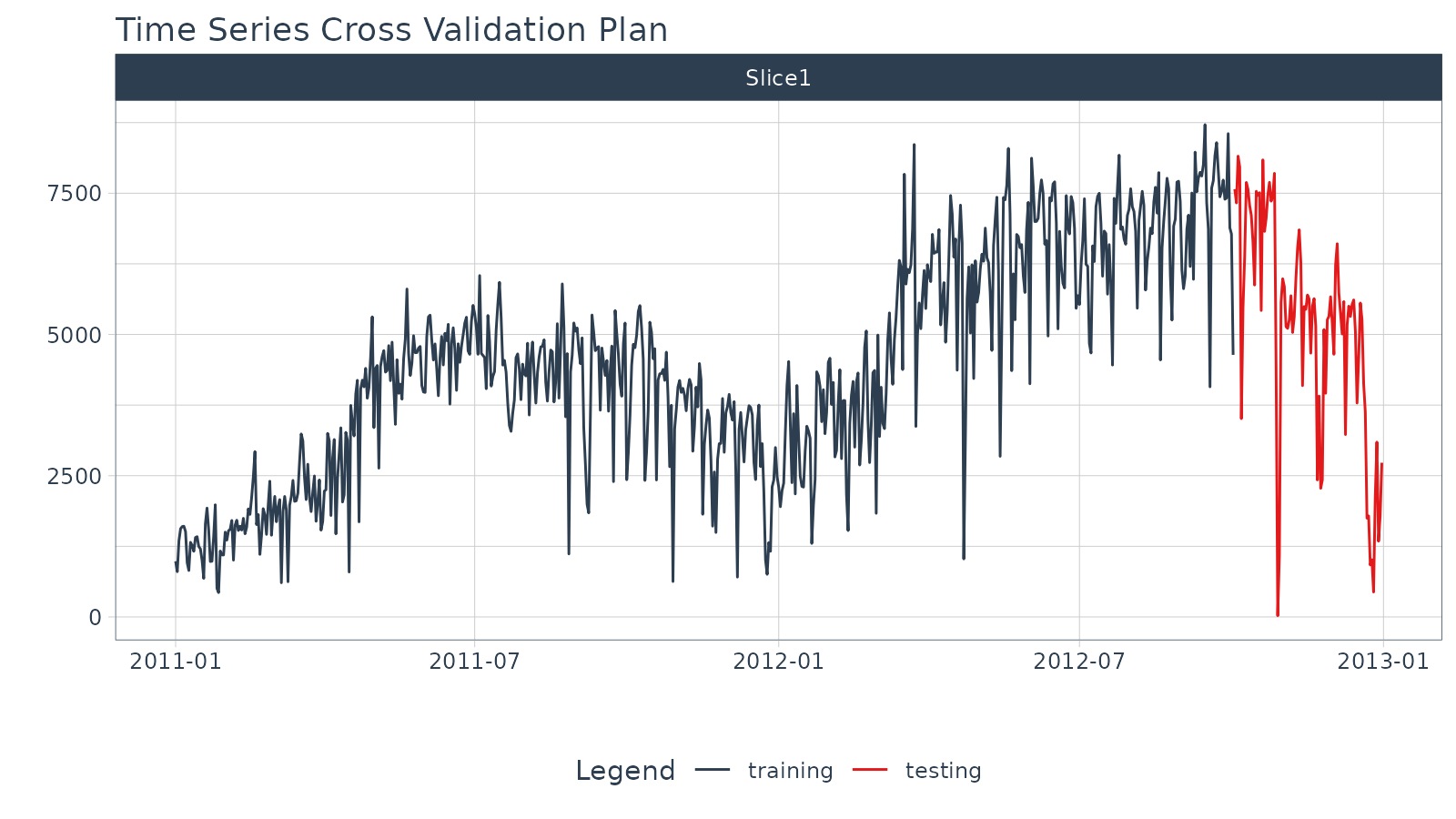

Modeling

Machine learning models are more complex than univariate models (e.g. ARIMA, Exponential Smoothing). This complexity typically requires a workflow (sometimes called a pipeline in other languages). The general process goes like this:

Create Preprocessing Recipe
Create Model Specifications
Use Workflow to combine Model Spec and Preprocessing, and Fit Model

Recipe Preprocessing Specification

The first step is to add the time series signature to the training set, which will be used this to learn the patterns. New in timetk 0.1.3 is integration with the recipes R package:

The recipes package allows us to add preprocessing steps that are applied sequentially as part of a data transformation pipeline.
The timetk has step_timeseries_signature(), which is used to add a number of features that can help machine learning models.

library(recipes)
# Add time series signature
recipe_spec_timeseries <- recipe(value ~ ., data = training(splits)) %>%
    step_timeseries_signature(date)

We can see what happens when we apply a prepared recipe prep() using the bake() function. Many new columns were added from the timestamp “date” feature. These are features we can use in our machine learning models.

bake(prep(recipe_spec_timeseries), new_data = training(splits))

## # A tibble: 641 × 29
##    date       value date_index.num date_year date_year.iso date_half
##    <date>     <dbl>          <dbl>     <int>         <int>     <int>
##  1 2011-01-01   985     1293840000      2011          2010         1
##  2 2011-01-02   801     1293926400      2011          2010         1
##  3 2011-01-03  1349     1294012800      2011          2011         1
##  4 2011-01-04  1562     1294099200      2011          2011         1
##  5 2011-01-05  1600     1294185600      2011          2011         1
##  6 2011-01-06  1606     1294272000      2011          2011         1
##  7 2011-01-07  1510     1294358400      2011          2011         1
##  8 2011-01-08   959     1294444800      2011          2011         1
##  9 2011-01-09   822     1294531200      2011          2011         1
## 10 2011-01-10  1321     1294617600      2011          2011         1
## # ℹ 631 more rows
## # ℹ 23 more variables: date_quarter <int>, date_month <int>,
## #   date_month.xts <int>, date_month.lbl <ord>, date_day <int>,
## #   date_hour <int>, date_minute <int>, date_second <int>, date_hour12 <int>,
## #   date_am.pm <int>, date_wday <int>, date_wday.xts <int>,
## #   date_wday.lbl <ord>, date_mday <int>, date_qday <int>, date_yday <int>,
## #   date_mweek <int>, date_week <int>, date_week.iso <int>, date_week2 <int>, …

Next, I apply various preprocessing steps to improve the modeling behavior. If you wish to learn more, I have an Advanced Time Series course that will help you learn these techniques.

recipe_spec_final <- recipe_spec_timeseries %>%
    step_fourier(date, period = 365, K = 5) %>%
    step_rm(date) %>%
    step_rm(contains("iso"), contains("minute"), contains("hour"),
            contains("am.pm"), contains("xts")) %>%
    step_normalize(contains("index.num"), date_year) %>%
    step_dummy(contains("lbl"), one_hot = TRUE) 

juice(prep(recipe_spec_final))

## # A tibble: 641 × 47
##    value date_index.num date_year date_half date_quarter date_month date_day
##    <dbl>          <dbl>     <dbl>     <int>        <int>      <int>    <int>
##  1   985          -1.73    -0.869         1            1          1        1
##  2   801          -1.72    -0.869         1            1          1        2
##  3  1349          -1.72    -0.869         1            1          1        3
##  4  1562          -1.71    -0.869         1            1          1        4
##  5  1600          -1.71    -0.869         1            1          1        5
##  6  1606          -1.70    -0.869         1            1          1        6
##  7  1510          -1.70    -0.869         1            1          1        7
##  8   959          -1.69    -0.869         1            1          1        8
##  9   822          -1.68    -0.869         1            1          1        9
## 10  1321          -1.68    -0.869         1            1          1       10
## # ℹ 631 more rows
## # ℹ 40 more variables: date_second <int>, date_wday <int>, date_mday <int>,
## #   date_qday <int>, date_yday <int>, date_mweek <int>, date_week <int>,
## #   date_week2 <int>, date_week3 <int>, date_week4 <int>, date_mday7 <int>,
## #   date_sin365_K1 <dbl>, date_cos365_K1 <dbl>, date_sin365_K2 <dbl>,
## #   date_cos365_K2 <dbl>, date_sin365_K3 <dbl>, date_cos365_K3 <dbl>,
## #   date_sin365_K4 <dbl>, date_cos365_K4 <dbl>, date_sin365_K5 <dbl>, …

Model Specification

Next, let’s create a model specification. We’ll use a Elastic Net penalized regression via the glmnet package.

model_spec_lm <- linear_reg(
    mode = "regression", 
    penalty = 0.1
) %>%
    set_engine("glmnet")

Workflow

We can mary up the preprocessing recipe and the model using a workflow().

workflow_lm <- workflow() %>%
    add_recipe(recipe_spec_final) %>%
    add_model(model_spec_lm)

workflow_lm

## ══ Workflow ════════════════════════════════════════════════════════════════════
## Preprocessor: Recipe
## Model: linear_reg()
## 
## ── Preprocessor ────────────────────────────────────────────────────────────────
## 6 Recipe Steps
## 
## • step_timeseries_signature()
## • step_fourier()
## • step_rm()
## • step_rm()
## • step_normalize()
## • step_dummy()
## 
## ── Model ───────────────────────────────────────────────────────────────────────
## Linear Regression Model Specification (regression)
## 
## Main Arguments:
##   penalty = 0.1
## 
## Computational engine: glmnet

Training

The workflow can be trained with the fit() function.

if (requireNamespace("glmnet")) {
  workflow_fit_lm <- workflow_lm %>% fit(data = training(splits))
}

Hyperparameter Tuning

Linear regression has no parameters. Therefore, this step is not needed. More complex models have hyperparameters that require tuning. Algorithms include:

Elastic Net
XGBoost
Random Forest
Support Vector Machine (SVM)
K-Nearest Neighbors
Multivariate Adaptive Regression Spines (MARS)

If you would like to learn how to tune these models for time series, then join the waitlist for my advanced Time Series Analysis & Forecasting Course.

Forecasting with Modeltime

The Modeltime Workflow is designed to speed up model evaluation and selection. Now that we have several time series models, let’s analyze them and forecast the future with the modeltime package.

Modeltime Table

The Modeltime Table organizes the models with IDs and creates generic descriptions to help us keep track of our models. Let’s add the models to a modeltime_table().

if (rlang::is_installed("modeltime")) {
  model_table <- modeltime::modeltime_table(
  workflow_fit_lm
) 

model_table
}

## # Modeltime Table
## # A tibble: 1 × 3
##   .model_id .model     .model_desc
##       <int> <list>     <chr>      
## 1         1 <workflow> GLMNET

Calibration

Model Calibration is used to quantify error and estimate confidence intervals. We’ll perform model calibration on the out-of-sample data (aka. the Testing Set) with the modeltime::modeltime_calibrate() function. Two new columns are generated (“.type” and “.calibration_data”), the most important of which is the “.calibration_data”. This includes the actual values, fitted values, and residuals for the testing set.

calibration_table <- model_table %>%
  modeltime::modeltime_calibrate(testing(splits))

calibration_table

## # Modeltime Table
## # A tibble: 1 × 5
##   .model_id .model     .model_desc .type .calibration_data
##       <int> <list>     <chr>       <chr> <list>           
## 1         1 <workflow> GLMNET      Test  <tibble [90 × 4]>

Forecast (Testing Set)

With calibrated data, we can visualize the testing predictions (forecast).

Use modeltime::modeltime_forecast() to generate the forecast data for the testing set as a tibble.
Use modeltime::plot_modeltime_forecast() to visualize the results in interactive and static plot formats.

calibration_table %>%
  modeltime::modeltime_forecast(actual_data = bike_transactions_tbl) %>%
  modeltime::plot_modeltime_forecast(.interactive = interactive)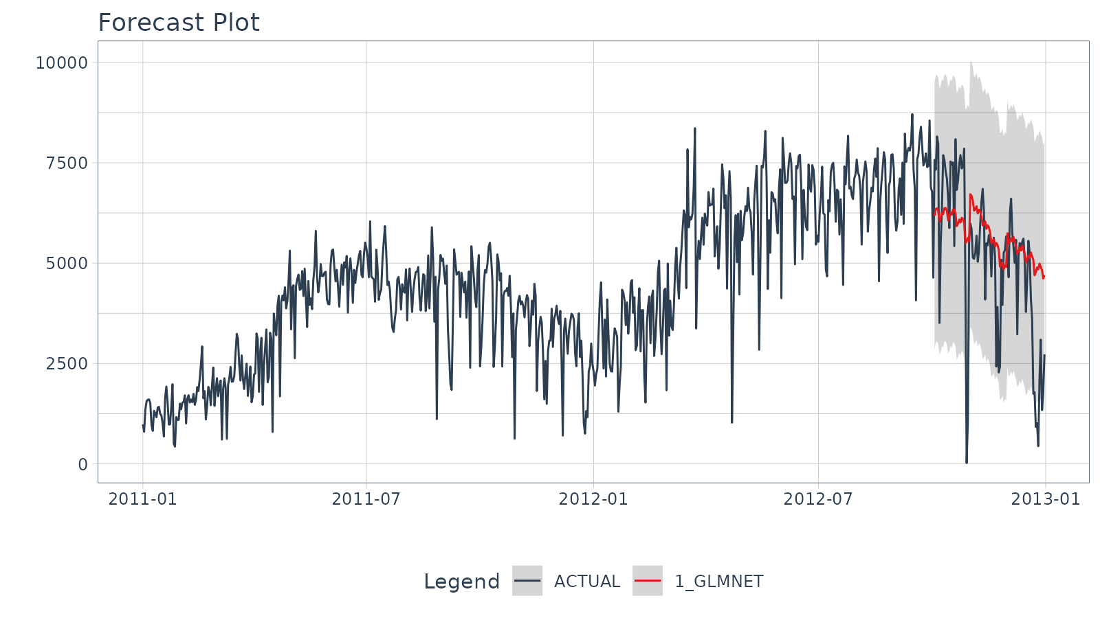

Accuracy (Testing Set)

Next, calculate the testing accuracy to compare the models.

Use modeltime::modeltime_accuracy() to generate the out-of-sample accuracy metrics as a tibble.
Use modeltime::table_modeltime_accuracy() to generate interactive and static

calibration_table %>%
  modeltime::modeltime_accuracy() %>%
  modeltime::table_modeltime_accuracy(.interactive = interactive)

.model_id	.model_desc	.type	mae	mape	mase	smape	rmse	rsq
Accuracy Table
1	GLMNET	Test	1244.11	331.5	1.34	29.2	1689.76	0.47

Refit and Forecast Forward

Refitting is a best-practice before forecasting the future.

modeltime::modeltime_refit(): We re-train on full data (bike_transactions_tbl)
modeltime::modeltime_forecast(): For models that only depend on the “date” feature, we can use h (horizon) to forecast forward. Setting h = "12 months" forecasts then next 12-months of data.

calibration_table %>%
  modeltime::modeltime_refit(bike_transactions_tbl) %>%
  modeltime::modeltime_forecast(h = "12 months", actual_data = bike_transactions_tbl) %>%
  modeltime::plot_modeltime_forecast(.interactive = interactive)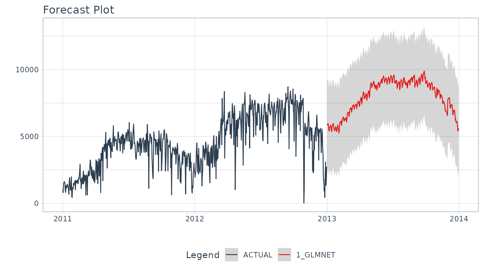

Summary

Timetk is part of the amazing Modeltime Ecosystem for time series forecasting. But it can take a long time to learn:

Many algorithms
Ensembling and Resampling
Feature Engineering
Machine Learning
Deep Learning
Scalable Modeling: 10,000+ time series

Your probably thinking how am I ever going to learn time series forecasting. Here’s the solution that will save you years of struggling.

Take the High-Performance Forecasting Course

Become the forecasting expert for your organization

High-Performance Time Series Course

Time Series is Changing

Time series is changing. Businesses now need 10,000+ time series forecasts every day. This is what I call a High-Performance Time Series Forecasting System (HPTSF) - Accurate, Robust, and Scalable Forecasting.

High-Performance Forecasting Systems will save companies by improving accuracy and scalability. Imagine what will happen to your career if you can provide your organization a “High-Performance Time Series Forecasting System” (HPTSF System).

How to Learn High-Performance Time Series Forecasting

I teach how to build a HPTFS System in my High-Performance Time Series Forecasting Course. You will learn:

Time Series Machine Learning (cutting-edge) with Modeltime - 30+ Models (Prophet, ARIMA, XGBoost, Random Forest, & many more)
Deep Learning with GluonTS (Competition Winners)
Time Series Preprocessing, Noise Reduction, & Anomaly Detection
Feature engineering using lagged variables & external regressors
Hyperparameter Tuning
Time series cross-validation
Ensembling Multiple Machine Learning & Univariate Modeling Techniques (Competition Winner)
Scalable Forecasting - Forecast 1000+ time series in parallel
and more.

Become the Time Series Expert for your organization.

Take the High-Performance Time Series Forecasting Course

Matt Dancho

2024-01-04