Time Series Data Wrangling

Time series data wrangling is an essential skill for any forecaster. timetk includes the essential data wrangling tools. In this tutorial, we’ll cover:

Summarise by Time - For time-based aggregations
Filter by Time - For complex time-based filtering
Pad by Time - For filling in gaps and going from low to high frequency
Slidify - For turning any function into a sliding (rolling) function

Additional concepts covered:

Imputation - Needed for Padding (See Low to High Frequency)
Advanced Filtering - Using the new add time %+time infix operation (See Padding Data: Low to High Frequency)
Visualization - plot_time_series() for all visualizations

Libraries

Load the following libraries.

library(dplyr)
library(tidyr)
library(timetk)

Data

This tutorial will use the FANG dataset:

Daily
Irregular (missing business holidays and weekends)
4 groups (FB, AMZN, NFLX, and GOOG).

FANG

## # A tibble: 4,032 × 8
##    symbol date        open  high   low close    volume adjusted
##    <chr>  <date>     <dbl> <dbl> <dbl> <dbl>     <dbl>    <dbl>
##  1 FB     2013-01-02  27.4  28.2  27.4  28    69846400     28  
##  2 FB     2013-01-03  27.9  28.5  27.6  27.8  63140600     27.8
##  3 FB     2013-01-04  28.0  28.9  27.8  28.8  72715400     28.8
##  4 FB     2013-01-07  28.7  29.8  28.6  29.4  83781800     29.4
##  5 FB     2013-01-08  29.5  29.6  28.9  29.1  45871300     29.1
##  6 FB     2013-01-09  29.7  30.6  29.5  30.6 104787700     30.6
##  7 FB     2013-01-10  30.6  31.5  30.3  31.3  95316400     31.3
##  8 FB     2013-01-11  31.3  32.0  31.1  31.7  89598000     31.7
##  9 FB     2013-01-14  32.1  32.2  30.6  31.0  98892800     31.0
## 10 FB     2013-01-15  30.6  31.7  29.9  30.1 173242600     30.1
## # ℹ 4,022 more rows

The adjusted column contains the adjusted closing prices for each day.

FANG %>%
  group_by(symbol) %>%
  plot_time_series(date, adjusted, .facet_ncol = 2, .interactive = FALSE)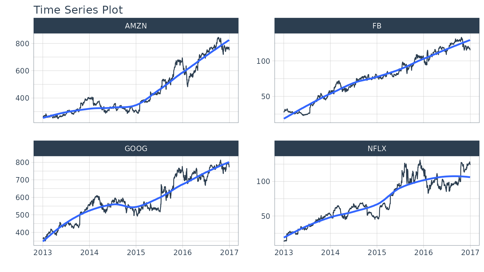

The volume column contains the trade volume (number of times the stock was transacted) for the day.

FANG %>%
  group_by(symbol) %>%
  plot_time_series(date, volume, .facet_ncol = 2, .interactive = FALSE)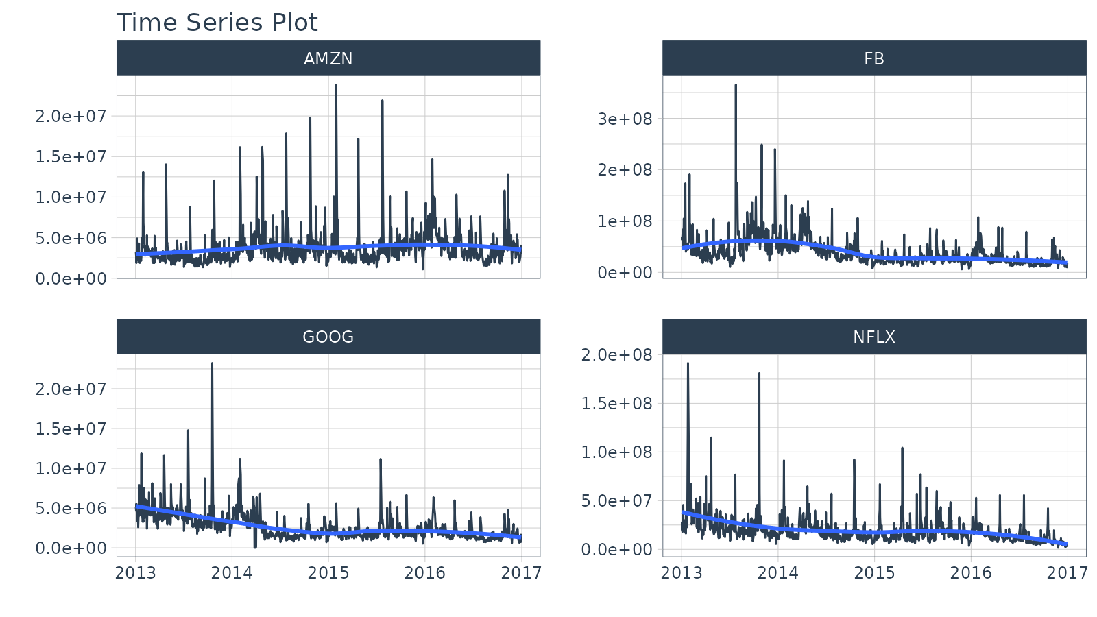

Summarize by Time

summarise_by_time() aggregates by a period. It’s great for:

Period Aggregation - sum()
Period Smoothing - mean(), first(), last()

Period Summarization

Objective: Get the total trade volume by quarter

Use sum()
Aggregate using .by = "quarter"

FANG %>%
  group_by(symbol) %>%
  summarise_by_time(
    date, 
    .by    = "quarter",
    volume = sum(volume)
  ) %>%
  plot_time_series(date, volume, .facet_ncol = 2, .interactive = FALSE, .y_intercept = 0)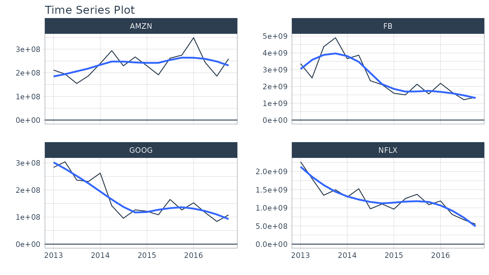

Period Smoothing

Objective: Get the first value in each month

We can use first() to get the first value, which has the effect of reducing the data (i.e. smoothing). We could use mean() or median().
Use the summarization by time: .by = "month" to aggregate by month.

FANG %>%
  group_by(symbol) %>%
  summarise_by_time(
    date, 
    .by = "month",
    adjusted = first(adjusted)
  ) %>%
  plot_time_series(date, adjusted, .facet_ncol = 2, .interactive = FALSE)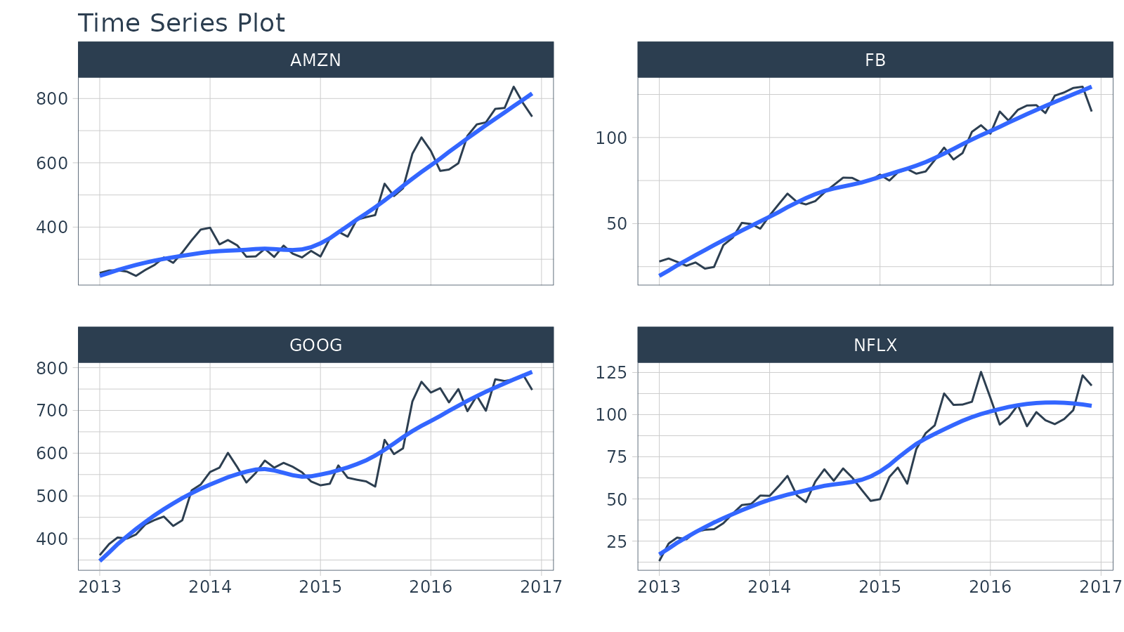

Filter By Time

Used to quickly filter a continuous time range.

Time Range Filtering

Objective: Get the adjusted stock prices in the 3rd quarter of 2013.

.start_date = "2013-09": Converts to “2013-09-01
.end_date = "2013": Converts to “2013-12-31
A more advanced example of filtering using %+time and %-time is shown in “Padding Data: Low to High Frequency”.

FANG %>%
  group_by(symbol) %>%
  filter_by_time(date, "2013-09", "2013") %>%
  plot_time_series(date, adjusted, .facet_ncol = 2, .interactive = FALSE)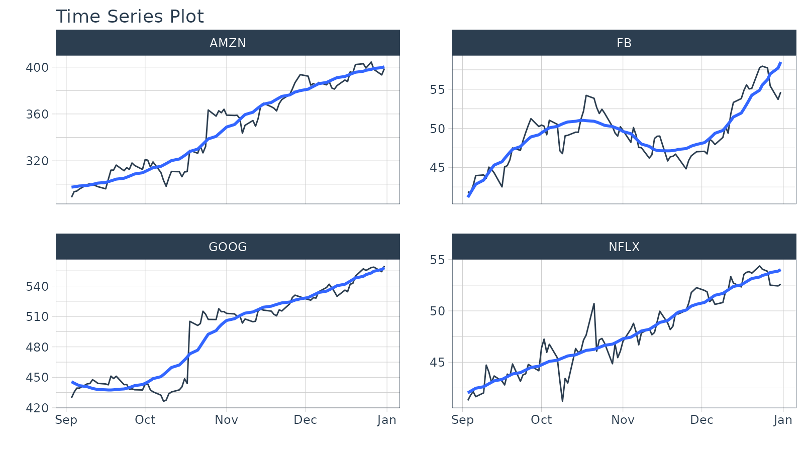

Padding Data

Used to fill in (pad) gaps and to go from from low frequency to high frequency. This function uses the awesome padr library for filling and expanding timestamps.

Fill in Gaps

Objective: Make an irregular series regular.

We will leave padded values as NA.
We can add a value using .pad_value or we can impute using a function like ts_impute_vec() (shown next).

FANG %>%
  group_by(symbol) %>%
  pad_by_time(date, .by = "auto") # Guesses .by = "day"

## pad applied on the interval: day

## # A tibble: 5,836 × 8
## # Groups:   symbol [4]
##    symbol date        open  high   low close  volume adjusted
##    <chr>  <date>     <dbl> <dbl> <dbl> <dbl>   <dbl>    <dbl>
##  1 AMZN   2013-01-02  256.  258.  253.  257. 3271000     257.
##  2 AMZN   2013-01-03  257.  261.  256.  258. 2750900     258.
##  3 AMZN   2013-01-04  258.  260.  257.  259. 1874200     259.
##  4 AMZN   2013-01-05   NA    NA    NA    NA       NA      NA 
##  5 AMZN   2013-01-06   NA    NA    NA    NA       NA      NA 
##  6 AMZN   2013-01-07  263.  270.  263.  268. 4910000     268.
##  7 AMZN   2013-01-08  267.  269.  264.  266. 3010700     266.
##  8 AMZN   2013-01-09  268.  270.  265.  266. 2265600     266.
##  9 AMZN   2013-01-10  269.  269.  262.  265. 2863400     265.
## 10 AMZN   2013-01-11  265.  268.  264.  268. 2413300     268.
## # ℹ 5,826 more rows

Low to High Frequency

Objective: Go from Daily to Hourly timestamp intervals for 1 month from the start date. Impute the missing values.

.by = "hour" pads from daily to hourly
Imputation of hourly data is accomplished with ts_impute_vec(), which performs linear interpolation when period = 1.
Filtering is accomplished using:
- “start”: A special keyword that signals the start of a series
- FIRST(date) %+time% "1 month": Selecting the first date in the sequence then using a special infix operation, %+time%, called “add time”. In this case I add “1 month”.

FANG %>%
  group_by(symbol) %>%
  pad_by_time(date, .by = "hour") %>%
  mutate_at(vars(open:adjusted), .funs = ts_impute_vec, period = 1) %>%
  filter_by_time(date, "start", first(date) %+time% "1 month") %>%
  plot_time_series(date, adjusted, .facet_ncol = 2, .interactive = FALSE)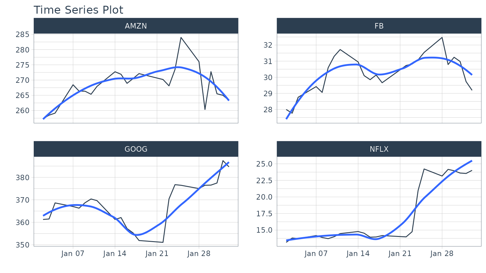

Sliding (Rolling) Calculations

We have a new function, slidify() that turns any function into a sliding (rolling) window function. It takes concepts from tibbletime::rollify() and it improves them with the R package slider.

Rolling Mean

Objective: Calculate a “centered” simple rolling average with partial window rolling and the start and end windows.

slidify() turns the mean() function into a rolling average.

# Make the rolling function
roll_avg_30 <- slidify(.f = mean, .period = 30, .align = "center", .partial = TRUE)

# Apply the rolling function
FANG %>%
  select(symbol, date, adjusted) %>%
  group_by(symbol) %>%
  # Apply Sliding Function
  mutate(rolling_avg_30 = roll_avg_30(adjusted)) %>%
  tidyr::pivot_longer(cols = c(adjusted, rolling_avg_30)) %>%
  plot_time_series(date, value, .color_var = name,
                   .facet_ncol = 2, .smooth = FALSE, 
                   .interactive = FALSE)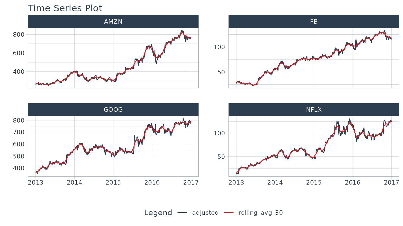

For simple rolling calculations (rolling average), we can accomplish this operation faster with slidify_vec() - A vectorized rolling function for simple summary rolls (e.g. mean(), sd(), sum(), etc)

FANG %>%
  select(symbol, date, adjusted) %>%
  group_by(symbol) %>%
  # Apply roll apply Function
  mutate(rolling_avg_30 = slidify_vec(adjusted,  ~ mean(.), 
                                      .period = 30, .partial = TRUE))

## # A tibble: 4,032 × 4
## # Groups:   symbol [4]
##    symbol date       adjusted rolling_avg_30
##    <chr>  <date>        <dbl>          <dbl>
##  1 FB     2013-01-02     28             30.0
##  2 FB     2013-01-03     27.8           30.1
##  3 FB     2013-01-04     28.8           30.2
##  4 FB     2013-01-07     29.4           30.2
##  5 FB     2013-01-08     29.1           30.3
##  6 FB     2013-01-09     30.6           30.3
##  7 FB     2013-01-10     31.3           30.3
##  8 FB     2013-01-11     31.7           30.2
##  9 FB     2013-01-14     31.0           30.1
## 10 FB     2013-01-15     30.1           30.1
## # ℹ 4,022 more rows

Rolling Regression

Objective: Calculate a rolling regression.

This is a complex sliding (rolling) calculation that requires multiple columns to be involved.
slidify() is built for this.
Use the multi-variable purrr ..1, ..2, ..3, etc notation to setup a function

# Rolling regressions are easy to implement using `.unlist = FALSE`
lm_roll <- slidify(~ lm(..1 ~ ..2 + ..3), .period = 90, 
                   .unlist = FALSE, .align = "right")


FANG %>%
  select(symbol, date, adjusted, volume) %>%
  group_by(symbol) %>%
  mutate(numeric_date = as.numeric(date)) %>%
  # Apply rolling regression
  mutate(rolling_lm = lm_roll(adjusted, volume, numeric_date)) %>%
  filter(!is.na(rolling_lm))

## # A tibble: 3,676 × 6
## # Groups:   symbol [4]
##    symbol date       adjusted   volume numeric_date rolling_lm
##    <chr>  <date>        <dbl>    <dbl>        <dbl> <list>    
##  1 FB     2013-05-10     26.7 30847100        15835 <lm>      
##  2 FB     2013-05-13     26.8 29068800        15838 <lm>      
##  3 FB     2013-05-14     27.1 24930300        15839 <lm>      
##  4 FB     2013-05-15     26.6 30299800        15840 <lm>      
##  5 FB     2013-05-16     26.1 35499100        15841 <lm>      
##  6 FB     2013-05-17     26.2 29462700        15842 <lm>      
##  7 FB     2013-05-20     25.8 42402900        15845 <lm>      
##  8 FB     2013-05-21     25.7 26261300        15846 <lm>      
##  9 FB     2013-05-22     25.2 45314500        15847 <lm>      
## 10 FB     2013-05-23     25.1 37663100        15848 <lm>      
## # ℹ 3,666 more rows

Learning More

My Talk on High-Performance Time Series Forecasting

Time series is changing. Businesses now need 10,000+ time series forecasts every day.

High-Performance Forecasting Systems will save companies MILLIONS of dollars. Imagine what will happen to your career if you can provide your organization a “High-Performance Time Series Forecasting System” (HPTSF System).

I teach how to build a HPTFS System in my High-Performance Time Series Forecasting Course. If interested in learning Scalable High-Performance Forecasting Strategies then take my course. You will learn:

Time Series Machine Learning (cutting-edge) with Modeltime - 30+ Models (Prophet, ARIMA, XGBoost, Random Forest, & many more)
NEW - Deep Learning with GluonTS (Competition Winners)
Time Series Preprocessing, Noise Reduction, & Anomaly Detection
Feature engineering using lagged variables & external regressors
Hyperparameter Tuning
Time series cross-validation
Ensembling Multiple Machine Learning & Univariate Modeling Techniques (Competition Winner)
Scalable Forecasting - Forecast 1000+ time series in parallel
and more.

Unlock the High-Performance Time Series Forecasting Course

Matt Dancho

2024-01-04