Frequency and Trend Selection
Source:vignettes/TK06_Automatic_Frequency_And_Trend_Selection.Rmd
TK06_Automatic_Frequency_And_Trend_Selection.RmdFrequency and trend cycles are used in many time
series applications including Seasonal ARIMA (SARIMA) forecasting and
STL Decomposition. timetk includes functionality for
Automatic Frequency and Trend Selection. These tools
use only the the timestamp information to make logical guesses about the
frequency and trend.
Data
Daily Irregular Data
The daily stock prices of Facebook from 2013 to 2016. Note that trading days only occur on “business days” (non-weekends and non-business-holidays).
## # A tibble: 1,008 × 8
##    symbol date        open  high   low close    volume adjusted
##    <chr>  <date>     <dbl> <dbl> <dbl> <dbl>     <dbl>    <dbl>
##  1 FB     2013-01-02  27.4  28.2  27.4  28    69846400     28
##  2 FB     2013-01-03  27.9  28.5  27.6  27.8  63140600     27.8
##  3 FB     2013-01-04  28.0  28.9  27.8  28.8  72715400     28.8
##  4 FB     2013-01-07  28.7  29.8  28.6  29.4  83781800     29.4
##  5 FB     2013-01-08  29.5  29.6  28.9  29.1  45871300     29.1
##  6 FB     2013-01-09  29.7  30.6  29.5  30.6 104787700     30.6
##  7 FB     2013-01-10  30.6  31.5  30.3  31.3  95316400     31.3
##  8 FB     2013-01-11  31.3  32.0  31.1  31.7  89598000     31.7
##  9 FB     2013-01-14  32.1  32.2  30.6  31.0  98892800     31.0
## 10 FB     2013-01-15  30.6  31.7  29.9  30.1 173242600     30.1
## # ℹ 998 more rows
Sub-Daily Data
Taylor’s Energy Demand data at a 30-minute timestamp interval.
taylor_30_min## # A tibble: 4,032 × 2
## date value
## <dttm> <dbl>
## 1 2000-06-05 00:00:00 22262
## 2 2000-06-05 00:30:00 21756
## 3 2000-06-05 01:00:00 22247
## 4 2000-06-05 01:30:00 22759
## 5 2000-06-05 02:00:00 22549
## 6 2000-06-05 02:30:00 22313
## 7 2000-06-05 03:00:00 22128
## 8 2000-06-05 03:30:00 21860
## 9 2000-06-05 04:00:00 21751
## 10 2000-06-05 04:30:00 21336
## # ℹ 4,022 more rowsApplications
An example of where automatic frequency detection occurs is in the
plot_stl_diagnostics() function.
taylor_30_min %>%
    plot_stl_diagnostics(date, value,
                         .frequency = "auto", .trend = "auto",
                         .interactive = FALSE)
## frequency = 48 observations per 1 day## trend = 672 observations per 14 days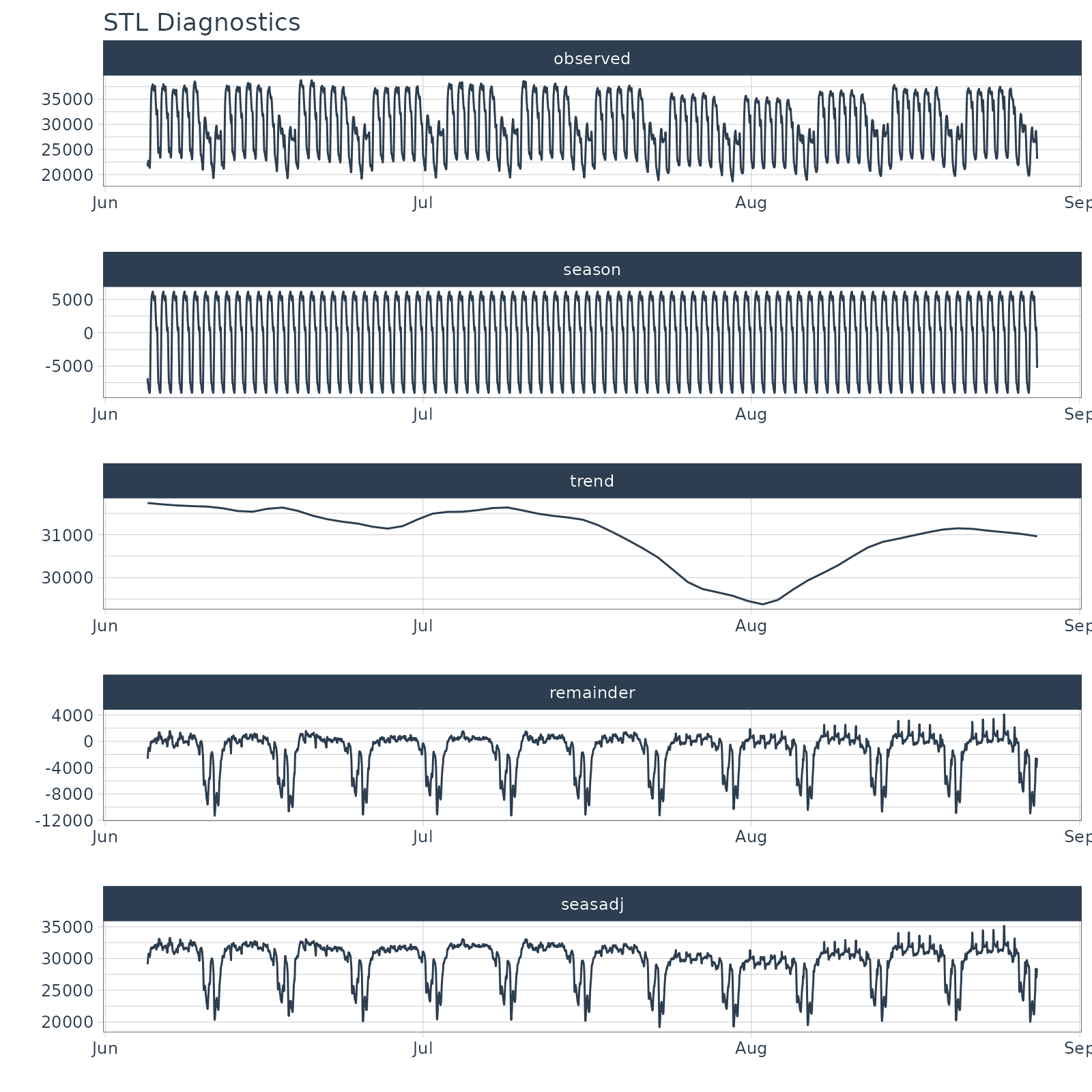
Automatic Frequency & Trend Selection
Specifying a Frequency or Trend
The period argument has three basic options for
returning a frequency. Options include:
- “auto”: A target frequency is determined using a pre-defined Time Scale Template (see below).
- time-based duration: (e.g. “7 days” or “2 quarters” per cycle)
- numeric number of observations: (e.g. 5 for 5 observations per cycle)
Frequency
A frequency is loosely defined as the number of observations that comprise a cycle in a data set.
Using tk_get_frequency(), we can pick a number of
observations that will roughly define a frequency for the series.
Daily Irregular Data
Because FB_tbl is irregular (weekends and holidays are
not present), the frequency selected is weekly but each week is only
5-days typically. So 5 is selected.
FB_tbl %>% tk_index() %>% tk_get_frequency(period = "auto")## frequency = 5 observations per 1 week## [1] 5Sub-Daily Data
This works as well for a sub-daily time series. Here we’ll use
taylor_30_min for a 30-minute timestamp series. The
frequency selected is 48 because there are 48 timestamps (observations)
in 1 day for the 30-minute cycle.
taylor_30_min %>% tk_index() %>% tk_get_frequency("1 day")## frequency = 48 observations per 1 day## [1] 48Trend
The trend is loosely defined as time span that can be aggregated across to visualize the central tendency of the data.
Using tk_get_trend(), we can pick a number of
observations that will help describe a trend for the data.
Daily Irregular Data
Because FB_tbl is irregular (weekends and holidays are
not present), the trend selected is 3 months but each week is only
5-days typically. So 64 observations is selected.
FB_tbl %>% tk_index() %>% tk_get_trend(period = "auto")## trend = 64 observations per 3 months## [1] 64Sub-Daily Data
A 14-day (2 week) interval is selected for the “30-minute” interval data.
taylor_30_min %>% tk_index() %>% tk_get_trend("auto")## trend = 672 observations per 14 days## [1] 672Time Scale Template
A Time-Scale Template is used to get and
set the time scale template, which is used by
tk_get_frequency() and tk_get_trend() when
period = "auto".
The predefined template is stored in a function
tk_time_scale_template(). This is the default used by
timetk.
Accessing the Default Template
You can access the current template with
get_tk_time_scale_template().
## # A tibble: 8 × 3
##   time_scale frequency trend
##   <chr>      <chr>     <chr>
## 1 second     1 hour    12 hours
## 2 minute     1 day     14 days
## 3 hour       1 day     1 month
## 4 day        1 week    3 months
## 5 week       1 quarter 1 year
## 6 month      1 year    5 years
## 7 quarter    1 year    10 years
## 8 year       5 years   30 years
Changing the Default Template
You can modify the current template with
set_tk_time_scale_template().
Learning More
My Talk on High-Performance Time Series Forecasting
Time series is changing. Businesses now need 10,000+ time series forecasts every day.
High-Performance Forecasting Systems will save companies MILLIONS of dollars. Imagine what will happen to your career if you can provide your organization a “High-Performance Time Series Forecasting System” (HPTSF System).
I teach how to build a HPTFS System in my High-Performance Time Series Forecasting Course. If interested in learning Scalable High-Performance Forecasting Strategies then take my course. You will learn:
- Time Series Machine Learning (cutting-edge) with
Modeltime- 30+ Models (Prophet, ARIMA, XGBoost, Random Forest, & many more) - NEW - Deep Learning with
GluonTS(Competition Winners) - Time Series Preprocessing, Noise Reduction, & Anomaly Detection
- Feature engineering using lagged variables & external regressors
- Hyperparameter Tuning
- Time series cross-validation
- Ensembling Multiple Machine Learning & Univariate Modeling Techniques (Competition Winner)
- Scalable Forecasting - Forecast 1000+ time series in parallel
- and more.