Visualize STL Decomposition Features for One or More Time Series
Source:R/plot-stl_diagnostics.R
plot_stl_diagnostics.RdAn interactive and scalable function for visualizing time series STL Decomposition.
Plots are available in interactive plotly (default) and static ggplot2 format.
Usage
plot_stl_diagnostics(
  .data,
  .date_var,
  .value,
  .facet_vars = NULL,
  .feature_set = c("observed", "season", "trend", "remainder", "seasadj"),
  .frequency = "auto",
  .trend = "auto",
  .message = TRUE,
  .facet_scales = "free",
  .line_color = "#2c3e50",
  .line_size = 0.5,
  .line_type = 1,
  .line_alpha = 1,
  .title = "STL Diagnostics",
  .x_lab = "",
  .y_lab = "",
  .interactive = TRUE
)
Arguments
- .data
A
tibbleordata.framewith a time-based column- .date_var
A column containing either date or date-time values
- .value
A column containing numeric values
- .facet_vars
One or more grouping columns that broken out into
ggplot2facets. These can be selected usingtidyselect()helpers (e.gcontains()).- .feature_set
The STL decompositions to visualize. Select one or more of "observed", "season", "trend", "remainder", "seasadj".
- .frequency
Controls the seasonal adjustment (removal of seasonality). Input can be either "auto", a time-based definition (e.g. "2 weeks"), or a numeric number of observations per frequency (e.g. 10). Refer to
tk_get_frequency().- .trend
Controls the trend component. For STL, trend controls the sensitivity of the lowess smoother, which is used to remove the remainder.
- .message
A boolean. If
TRUE, will output information related to automatic frequency and trend selection (if applicable).- .facet_scales
Control facet x & y-axis ranges. Options include "fixed", "free", "free_y", "free_x"
- .line_color
Line color.
- .line_size
Line size.
- .line_type
Line type.
- .line_alpha
Line alpha (opacity). Range: (0, 1).
- .title
Plot title.
- .x_lab
Plot x-axis label
- .y_lab
Plot y-axis label
- .interactive
If TRUE, returns a
plotlyinteractive plot. If FALSE, returns a staticggplot2plot.
Details
The plot_stl_diagnostics() function generates a Seasonal-Trend-Loess decomposition.
The function is "tidy" in the sense that it works
on data frames and is designed to work with dplyr groups.
STL method:
The STL method implements time series decomposition using
the underlying stats::stl(). The decomposition separates the
"season" and "trend" components from
the "observed" values leaving the "remainder".
Frequency & Trend Selection
The user can control two parameters: .frequency and .trend.
The
.frequencyparameter adjusts the "season" component that is removed from the "observed" values.The
.trendparameter adjusts the trend window (t.windowparameter fromstl()) that is used.
The user may supply both .frequency
and .trend as time-based durations (e.g. "6 weeks") or numeric values
(e.g. 180) or "auto", which automatically selects the frequency and/or trend
based on the scale of the time series.
Examples
library(dplyr)
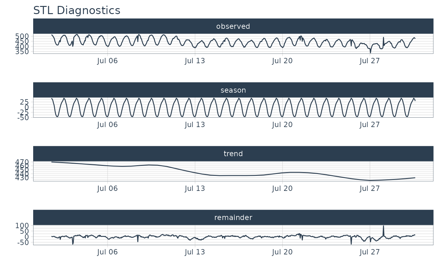
# ---- SINGLE TIME SERIES DECOMPOSITION ----
m4_hourly %>%
filter(id == "H10") %>%
plot_stl_diagnostics(
date, value,
# Set features to return, desired frequency and trend
.feature_set = c("observed", "season", "trend", "remainder"),
.frequency = "24 hours",
.trend = "1 week",
.interactive = FALSE)
#> frequency = 24 observations per 24 hours
#> trend = 168 observations per 1 week
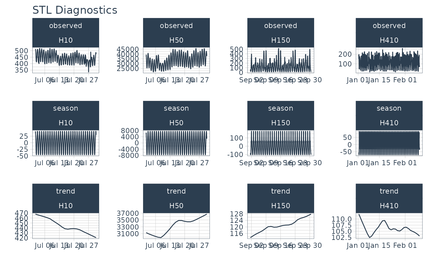
 # ---- GROUPS ----
m4_hourly %>%
group_by(id) %>%
plot_stl_diagnostics(
date, value,
.feature_set = c("observed", "season", "trend"),
.interactive = FALSE)
#> frequency = 24 observations per 1 day
#> trend = 336 observations per 14 days
#> frequency = 24 observations per 1 day
#> trend = 336 observations per 14 days
#> frequency = 24 observations per 1 day
#> trend = 336 observations per 14 days
#> frequency = 24 observations per 1 day
#> trend = 336 observations per 14 days
# ---- GROUPS ----
m4_hourly %>%
group_by(id) %>%
plot_stl_diagnostics(
date, value,
.feature_set = c("observed", "season", "trend"),
.interactive = FALSE)
#> frequency = 24 observations per 1 day
#> trend = 336 observations per 14 days
#> frequency = 24 observations per 1 day
#> trend = 336 observations per 14 days
#> frequency = 24 observations per 1 day
#> trend = 336 observations per 14 days
#> frequency = 24 observations per 1 day
#> trend = 336 observations per 14 days