Demand Forecasting

Timetk enables you to generate features from the time column of your data very easily. This tutorial showcases how easy it is to perform time series forecasting with pytimetk. The specific methods we will be using are:

• tk.augment_timeseries_signature(): Add 29 time series features to a DataFrame.
• tk.augment_lags(): Adds past values of a feature as a predictor
• tk.augment_rolling(): Calculates rolling window aggregates of a feature.
• tk.plot_timeseries(): Creates time series plots using different plotting engines such as Plotnine, Matplotlib, and Plotly.
• tk.future_frame(): Extend a DataFrame or GroupBy object with future dates.

1 Tutorial Setup

1.1 Load Packages

Load the following packages before proceeding with this tutorial.

Code

import pandas as pd
import numpy as np
import pytimetk as tk

from sklearn.ensemble import RandomForestRegressor

The tutorial is divided into three parts: We will first have a look at the Walmart dataset and perform some preprocessing. Secondly, we will create models based on different features, and see how the time features can be useful. Finally, we will solve the task of time series forecasting, using the features from augment_timeseries_signature, augment_lags, and augment_rolling, to predict future sales.

1.2 Load & Inspect dataset

The first thing we want to do is to load the dataset. It is a subset of the Walmart sales prediction Kaggle competition. You can get more insights about the dataset by following this link: walmart_sales_weekly. The most important thing to know about the dataset is that you are provided with some features like the fuel price or whether the week contains holidays and you are expected to predict the weekly sales column for 7 different departments of a given store. Of course, you also have the date for each week, and that is what we can leverage to create additional features.

Let us start by loading the dataset and cleaning it. Note that we also removed some columns due to * duplication of data * 0 variance * No future data available in current dataset.

Code

# We start by loading the dataset
# /walmart_sales_weekly.html
dset = tk.load_dataset('walmart_sales_weekly', parse_dates = ['Date'])

dset = dset.drop(columns=[
    'id', # This column can be removed as it is equivalent to 'Dept'
    'Store', # This column has only one possible value
    'Type', # This column has only one possible value
    'Size', # This column has only one possible value
    'MarkDown1', 'MarkDown2', 'MarkDown3', 'MarkDown4', 'MarkDown5',
    'IsHoliday', 'Temperature', 'Fuel_Price', 'CPI',
       'Unemployment'])

dset.head()

	Dept	Date	Weekly_Sales
0	1	2010-02-05	24924.50
1	1	2010-02-12	46039.49
2	1	2010-02-19	41595.55
3	1	2010-02-26	19403.54
4	1	2010-03-05	21827.90

We can plot the values of each department to get an idea of how the data looks like. Using the plot_timeseries method with a groupby allows us to create multiple plots by group.

Getting More Info: tk.plot_timeseries()

• Click here to see our Data Visualization Guide
• Use help(tk.plot_timeseries) to review additional helpful documentation.

Plotly

Code

sales_df = dset
fig = sales_df.groupby('Dept').plot_timeseries(
    date_column='Date',
    value_column='Weekly_Sales',
    facet_ncol = 2,
    x_axis_date_labels = "%Y",
    engine = 'plotly')
fig

Plotnine

Code

fig = sales_df.groupby('Dept').plot_timeseries(
    date_column='Date',
    value_column='Weekly_Sales',
    facet_ncol = 2,
    x_axis_date_labels = "%Y",
    engine = 'plotnine')
fig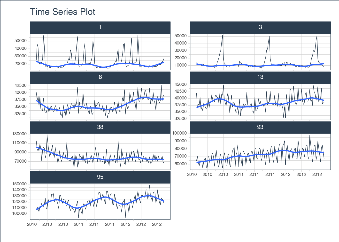

<Figure Size: (700 x 500)>

2 Create a Department Forecast Model

2.1 Making Future Dates Easier with tk.future_frame

When building machine learning models, we need to setup our dataframe to hold information about the future. This is the dataframe that will get passed to our model.predict() call. This is made easy with tk.future_frame().

Getting to know tk.future_frame()

Curious about the various options it provides?

• Click here to see our Data Wrangling Guide
• Use help(tk.future_frame) to review additional helpful documentation. And explore the plethora of possibilities!

Notice this function adds 5 weeks to our dateset for each department and fills in weekly sales with nulls. Previously our max date was 2012-10-26.

Code

print(sales_df.groupby('Dept').Date.max())

Dept
1    2012-10-26
3    2012-10-26
8    2012-10-26
13   2012-10-26
38   2012-10-26
93   2012-10-26
95   2012-10-26
Name: Date, dtype: datetime64[ns]

After applying our future frame, we can now see values 5 weeks in the future, and our dataframe has been extended to 2012-11-30 for all groups.

Code

sales_df_with_futureframe = sales_df \
    .groupby('Dept') \
    .future_frame(
        date_column = 'Date',
        length_out  = 5
    )

Code

sales_df_with_futureframe.groupby('Dept').Date.max()

Dept
1    2012-11-30
3    2012-11-30
8    2012-11-30
13   2012-11-30
38   2012-11-30
93   2012-11-30
95   2012-11-30
Name: Date, dtype: datetime64[ns]

2.2 Date Features with tk.augment_timeseries_signature

Machine Learning models generally cannot process raw date objects directly. Moreover, they lack an inherent understanding of the passage of time. This means that, without specific features, a model can’t differentiate between a January observation and a June one. To bridge this gap, the tk.augment_timeseries_signature function is invaluable. It generates 29 distinct date-oriented features suitable for model inputs.

Getting More Info: tk.augment_timeseries_signature(),tk.augment_lags(), tk.augment_rolling()

• Click here to see our Adding Features (Augmenting)
• Use help(tk.augment_timeseries_signature) help(tk.augment_lags) help(tk.augment_rolling) to review additional helpful documentation.
  

It’s crucial, however, to align these features with the granularity of your dataset. Given the weekly granularity of the Walmart dataset, any date attributes finer than ‘week’ should be excluded for relevance and efficiency.

Code

sales_df_dates = sales_df_with_futureframe.augment_timeseries_signature(date_column = 'Date')
sales_df_dates.head(10)

	Dept	Date	Weekly_Sales	Date_index_num	Date_year	Date_year_iso	Date_yearstart	Date_yearend	Date_leapyear	Date_half	...	Date_mday	Date_qday	Date_yday	Date_weekend	Date_hour	Date_minute	Date_second	Date_msecond	Date_nsecond	Date_am_pm
0	1	2010-02-05	24924.50	1265328000	2010	2010	0	0	0	1	...	5	36	36	0	0	0	0	0	0	am
1	1	2010-02-12	46039.49	1265932800	2010	2010	0	0	0	1	...	12	43	43	0	0	0	0	0	0	am
2	1	2010-02-19	41595.55	1266537600	2010	2010	0	0	0	1	...	19	50	50	0	0	0	0	0	0	am
3	1	2010-02-26	19403.54	1267142400	2010	2010	0	0	0	1	...	26	57	57	0	0	0	0	0	0	am
4	1	2010-03-05	21827.90	1267747200	2010	2010	0	0	0	1	...	5	64	64	0	0	0	0	0	0	am
5	1	2010-03-12	21043.39	1268352000	2010	2010	0	0	0	1	...	12	71	71	0	0	0	0	0	0	am
6	1	2010-03-19	22136.64	1268956800	2010	2010	0	0	0	1	...	19	78	78	0	0	0	0	0	0	am
7	1	2010-03-26	26229.21	1269561600	2010	2010	0	0	0	1	...	26	85	85	0	0	0	0	0	0	am
8	1	2010-04-02	57258.43	1270166400	2010	2010	0	0	0	1	...	2	2	92	0	0	0	0	0	0	am
9	1	2010-04-09	42960.91	1270771200	2010	2010	0	0	0	1	...	9	9	99	0	0	0	0	0	0	am

10 rows × 32 columns

Upon reviewing the generated features, it’s evident that certain attributes don’t align with the granularity of our dataset. For optimal results, features exhibiting no variance—like “Date_hour” due to the weekly nature of our data—should be omitted. We also spot redundant features, such as “Date_Month” and “Date_month_lbl”; both convey month information, albeit in different formats. To enhance clarity and computational efficiency, we’ll refine our dataset to include only the most relevant columns.

Additionally, we’ve eliminated certain categorical columns, which, although compatible with models like LightGBM and Catboost, demand extra processing for many tree-based ML models. While 1-hot encoding is a popular method for managing categorical data, it’s not typically recommended for date attributes. Instead, leveraging numeric date features directly, combined with the integration of Fourier features, can effectively capture cyclical patterns.

Code

sales_df_dates.glimpse()

<class 'pandas.core.frame.DataFrame'>: 1036 rows of 32 columns
Dept:               int64             [1, 1, 1, 1, 1, 1, 1, 1, 1, 1, 1,  ...
Date:               datetime64[ns]    [Timestamp('2010-02-05 00:00:00'), ...
Weekly_Sales:       float64           [24924.5, 46039.49, 41595.55, 1940 ...
Date_index_num:     int64             [1265328000, 1265932800, 126653760 ...
Date_year:          int64             [2010, 2010, 2010, 2010, 2010, 201 ...
Date_year_iso:      UInt32            [2010, 2010, 2010, 2010, 2010, 201 ...
Date_yearstart:     uint8             [0, 0, 0, 0, 0, 0, 0, 0, 0, 0, 0,  ...
Date_yearend:       uint8             [0, 0, 0, 0, 0, 0, 0, 0, 0, 0, 0,  ...
Date_leapyear:      uint8             [0, 0, 0, 0, 0, 0, 0, 0, 0, 0, 0,  ...
Date_half:          int64             [1, 1, 1, 1, 1, 1, 1, 1, 1, 1, 1,  ...
Date_quarter:       int64             [1, 1, 1, 1, 1, 1, 1, 1, 2, 2, 2,  ...
Date_quarteryear:   object            ['2010Q1', '2010Q1', '2010Q1', '20 ...
Date_quarterstart:  uint8             [0, 0, 0, 0, 0, 0, 0, 0, 0, 0, 0,  ...
Date_quarterend:    uint8             [0, 0, 0, 0, 0, 0, 0, 0, 0, 0, 0,  ...
Date_month:         int64             [2, 2, 2, 2, 3, 3, 3, 3, 4, 4, 4,  ...
Date_month_lbl:     object            ['February', 'February', 'February ...
Date_monthstart:    uint8             [0, 0, 0, 0, 0, 0, 0, 0, 0, 0, 0,  ...
Date_monthend:      uint8             [0, 0, 0, 0, 0, 0, 0, 0, 0, 0, 0,  ...
Date_yweek:         UInt32            [5, 6, 7, 8, 9, 10, 11, 12, 13, 14 ...
Date_mweek:         int64             [1, 2, 3, 4, 1, 2, 3, 4, 1, 2, 3,  ...
Date_wday:          int64             [5, 5, 5, 5, 5, 5, 5, 5, 5, 5, 5,  ...
Date_wday_lbl:      object            ['Friday', 'Friday', 'Friday', 'Fr ...
Date_mday:          int64             [5, 12, 19, 26, 5, 12, 19, 26, 2,  ...
Date_qday:          int64             [36, 43, 50, 57, 64, 71, 78, 85, 2 ...
Date_yday:          int64             [36, 43, 50, 57, 64, 71, 78, 85, 9 ...
Date_weekend:       int64             [0, 0, 0, 0, 0, 0, 0, 0, 0, 0, 0,  ...
Date_hour:          int64             [0, 0, 0, 0, 0, 0, 0, 0, 0, 0, 0,  ...
Date_minute:        int64             [0, 0, 0, 0, 0, 0, 0, 0, 0, 0, 0,  ...
Date_second:        int64             [0, 0, 0, 0, 0, 0, 0, 0, 0, 0, 0,  ...
Date_msecond:       int64             [0, 0, 0, 0, 0, 0, 0, 0, 0, 0, 0,  ...
Date_nsecond:       int64             [0, 0, 0, 0, 0, 0, 0, 0, 0, 0, 0,  ...
Date_am_pm:         object            ['am', 'am', 'am', 'am', 'am', 'am ...

Code

sales_df_dates = sales_df_dates[[
    'Date'
    ,'Dept'
    , 'Weekly_Sales'
    , 'Date_year'
    , 'Date_month'
    , 'Date_yweek'
    , 'Date_mweek'  
    ]]
sales_df_dates.tail(10)

	Date	Dept	Weekly_Sales	Date_year	Date_month	Date_yweek	Date_mweek
1026	2012-11-02	93	NaN	2012	11	44	1
1027	2012-11-09	93	NaN	2012	11	45	2
1028	2012-11-16	93	NaN	2012	11	46	3
1029	2012-11-23	93	NaN	2012	11	47	4
1030	2012-11-30	93	NaN	2012	11	48	5
1031	2012-11-02	95	NaN	2012	11	44	1
1032	2012-11-09	95	NaN	2012	11	45	2
1033	2012-11-16	95	NaN	2012	11	46	3
1034	2012-11-23	95	NaN	2012	11	47	4
1035	2012-11-30	95	NaN	2012	11	48	5

2.3 Lag Features with tk.augment_lags

As previously noted, it’s important to recognize that machine learning models lack inherent awareness of time, a vital consideration in time series modeling. Furthermore, these models operate under the assumption that each row is independent, meaning that the information from last month’s weekly sales is not inherently integrated into the prediction of next month’s sales target. To address this limitation, we incorporate additional features, such as lags, into the models to capture temporal dependencies. You can easily achieve this by employing the tk.augment_lags function.

Code

df_with_lags = sales_df_dates \
    .groupby('Dept') \
    .augment_lags(
        date_column  = 'Date',
        value_column = 'Weekly_Sales',
        lags         = [5,6,7,8,9]
    )
df_with_lags.head(5)

	Date	Dept	Weekly_Sales	Date_year	Date_month	Date_yweek	Date_mweek	Weekly_Sales_lag_5	Weekly_Sales_lag_6	Weekly_Sales_lag_7	Weekly_Sales_lag_8	Weekly_Sales_lag_9
0	2010-02-05	1	24924.50	2010	2	5	1	NaN	NaN	NaN	NaN	NaN
1	2010-02-12	1	46039.49	2010	2	6	2	NaN	NaN	NaN	NaN	NaN
2	2010-02-19	1	41595.55	2010	2	7	3	NaN	NaN	NaN	NaN	NaN
3	2010-02-26	1	19403.54	2010	2	8	4	NaN	NaN	NaN	NaN	NaN
4	2010-03-05	1	21827.90	2010	3	9	1	NaN	NaN	NaN	NaN	NaN

2.4 Rolling Lag Features with tk.augment_rolling

Another pivotal aspect of time series analysis involves the utilization of rolling lags. These operations facilitate computations within a moving time window, enabling the use of functions such as “mean” and “std” on these rolling windows. This can be achieved by invoking the tk.augment_rolling() function on grouped time series data. To execute this, we will initially gather all columns containing ‘lag’ in their names. We then apply this function to the lag values, as opposed to the weekly sales, since we lack future weekly sales data. By applying these functions to the lag values, we ensure the prevention of data leakage and maintain the adaptability of our method to unforeseen future data.

Code

lag_columns = [col for col in df_with_lags.columns if 'lag' in col]

df_with_rolling = df_with_lags \
    .groupby('Dept') \
    .augment_rolling(
        date_column  = 'Date',
        value_column = lag_columns,
        window  = 4,
        window_func = 'mean',
        threads = 1 # Change to -1 to use all available cores
    ) 
df_with_rolling[df_with_rolling.Dept ==1].head(10)

	Date	Dept	Weekly_Sales	Date_year	Date_month	Date_yweek	Date_mweek	Weekly_Sales_lag_5	Weekly_Sales_lag_6	Weekly_Sales_lag_7	Weekly_Sales_lag_8	Weekly_Sales_lag_9	Weekly_Sales_lag_5_rolling_mean_win_4	Weekly_Sales_lag_6_rolling_mean_win_4	Weekly_Sales_lag_7_rolling_mean_win_4	Weekly_Sales_lag_8_rolling_mean_win_4	Weekly_Sales_lag_9_rolling_mean_win_4
0	2010-02-05	1	24924.50	2010	2	5	1	NaN	NaN	NaN	NaN	NaN	NaN	NaN	NaN	NaN	NaN
0	2010-02-05	1	24924.50	2010	2	5	1	NaN	NaN	NaN	NaN	NaN	NaN	NaN	NaN	NaN	NaN
0	2010-02-05	1	24924.50	2010	2	5	1	NaN	NaN	NaN	NaN	NaN	NaN	NaN	NaN	NaN	NaN
0	2010-02-05	1	24924.50	2010	2	5	1	NaN	NaN	NaN	NaN	NaN	NaN	NaN	NaN	NaN	NaN
0	2010-02-05	1	24924.50	2010	2	5	1	NaN	NaN	NaN	NaN	NaN	NaN	NaN	NaN	NaN	NaN
1	2010-02-12	1	46039.49	2010	2	6	2	NaN	NaN	NaN	NaN	NaN	NaN	NaN	NaN	NaN	NaN
1	2010-02-12	1	46039.49	2010	2	6	2	NaN	NaN	NaN	NaN	NaN	NaN	NaN	NaN	NaN	NaN
1	2010-02-12	1	46039.49	2010	2	6	2	NaN	NaN	NaN	NaN	NaN	NaN	NaN	NaN	NaN	NaN
1	2010-02-12	1	46039.49	2010	2	6	2	NaN	NaN	NaN	NaN	NaN	NaN	NaN	NaN	NaN	NaN
1	2010-02-12	1	46039.49	2010	2	6	2	NaN	NaN	NaN	NaN	NaN	NaN	NaN	NaN	NaN	NaN

Notice when we add lag values to our dataframe, this creates several NA values. This is because when using lags, there will be some data that is not available early in our dataset.Thus as a result, NA values are introduced.

To simplify and clean up the process, we will remove these rows entirely since we already extracted some meaningful information from them (ie. lags, rolling lags).

Code

all_lag_columns = [col for col in df_with_rolling.columns if 'lag' in col]

df_no_nas = df_with_rolling \
    .dropna(subset=all_lag_columns, inplace=False)

df_no_nas.head()

	Date	Dept	Weekly_Sales	Date_year	Date_month	Date_yweek	Date_mweek	Weekly_Sales_lag_5	Weekly_Sales_lag_6	Weekly_Sales_lag_7	Weekly_Sales_lag_8	Weekly_Sales_lag_9	Weekly_Sales_lag_5_rolling_mean_win_4	Weekly_Sales_lag_6_rolling_mean_win_4	Weekly_Sales_lag_7_rolling_mean_win_4	Weekly_Sales_lag_8_rolling_mean_win_4	Weekly_Sales_lag_9_rolling_mean_win_4
12	2010-04-30	1	16555.11	2010	4	17	5	26229.21	22136.64	21043.39	21827.9	19403.54	22809.285	21102.8675	25967.595	32216.62	32990.77
12	2010-04-30	1	16555.11	2010	4	17	5	26229.21	22136.64	21043.39	21827.9	19403.54	22809.285	21102.8675	25967.595	32216.62	32990.77
12	2010-04-30	1	16555.11	2010	4	17	5	26229.21	22136.64	21043.39	21827.9	19403.54	22809.285	21102.8675	25967.595	32216.62	32990.77
12	2010-04-30	1	16555.11	2010	4	17	5	26229.21	22136.64	21043.39	21827.9	19403.54	22809.285	21102.8675	25967.595	32216.62	32990.77
12	2010-04-30	1	16555.11	2010	4	17	5	26229.21	22136.64	21043.39	21827.9	19403.54	22809.285	21102.8675	25967.595	32216.62	32990.77

We can call tk.glimpse() again to quickly see what features we still have available.

Code

df_no_nas.glimpse()

<class 'pandas.core.frame.DataFrame'>: 4760 rows of 17 columns
Date:                                   datetime64[ns]    [Timestamp('20 ...
Dept:                                   int64             [1, 1, 1, 1, 1 ...
Weekly_Sales:                           float64           [16555.11, 165 ...
Date_year:                              int64             [2010, 2010, 2 ...
Date_month:                             int64             [4, 4, 4, 4, 4 ...
Date_yweek:                             UInt32            [17, 17, 17, 1 ...
Date_mweek:                             int64             [5, 5, 5, 5, 5 ...
Weekly_Sales_lag_5:                     float64           [26229.21, 262 ...
Weekly_Sales_lag_6:                     float64           [22136.64, 221 ...
Weekly_Sales_lag_7:                     float64           [21043.39, 210 ...
Weekly_Sales_lag_8:                     float64           [21827.9, 2182 ...
Weekly_Sales_lag_9:                     float64           [19403.54, 194 ...
Weekly_Sales_lag_5_rolling_mean_win_4:  float64           [22809.285, 22 ...
Weekly_Sales_lag_6_rolling_mean_win_4:  float64           [21102.8675, 2 ...
Weekly_Sales_lag_7_rolling_mean_win_4:  float64           [25967.595, 25 ...
Weekly_Sales_lag_8_rolling_mean_win_4:  float64           [32216.6200000 ...
Weekly_Sales_lag_9_rolling_mean_win_4:  float64           [32990.7700000 ...

2.5 Training and Future Sets

Now that we have our training set built, we can start to train our regressor. To do so, let’s first do some model cleanup.

Split our data in to train and future sets.

Code

future = df_no_nas[df_no_nas.Weekly_Sales.isnull()]
train = df_no_nas[df_no_nas.Weekly_Sales.notnull()]

2.6 Model with regressor

We still have a datetime object in our training data. We will need to remove that before passing to our regressor. Let’s subset our column to just the features we want to use for modeling.

Code

train_columns = [ 
    'Dept'
    , 'Date_year'
    , 'Date_month'
    , 'Date_yweek'
    , 'Date_mweek'
    , 'Weekly_Sales_lag_5'
    , 'Weekly_Sales_lag_6'
    , 'Weekly_Sales_lag_7'
    , 'Weekly_Sales_lag_8'
    , 'Weekly_Sales_lag_5_rolling_mean_win_4'
    , 'Weekly_Sales_lag_6_rolling_mean_win_4'
    , 'Weekly_Sales_lag_7_rolling_mean_win_4'
    , 'Weekly_Sales_lag_8_rolling_mean_win_4'
    ]

X = train[train_columns]
y = train[['Weekly_Sales']]

model = RandomForestRegressor(random_state=123)
model = model.fit(X, y)

Now that we have a trained model, we can pass in our future frame to predict weekly sales.

Code

predicted_values = model.predict(future[train_columns])
future['y_pred'] = predicted_values

future.head(10)

	Date	Dept	Weekly_Sales	Date_year	Date_month	Date_yweek	Date_mweek	Weekly_Sales_lag_5	Weekly_Sales_lag_6	Weekly_Sales_lag_7	Weekly_Sales_lag_8	Weekly_Sales_lag_9	Weekly_Sales_lag_5_rolling_mean_win_4	Weekly_Sales_lag_6_rolling_mean_win_4	Weekly_Sales_lag_7_rolling_mean_win_4	Weekly_Sales_lag_8_rolling_mean_win_4	Weekly_Sales_lag_9_rolling_mean_win_4	y_pred
1001	2012-11-02	1	NaN	2012	11	44	1	18947.81	19251.50	19616.22	18322.37	16680.24	19034.475	18467.5825	17726.3075	17154.9275	16604.3150	26627.7378
1001	2012-11-02	1	NaN	2012	11	44	1	18947.81	19251.50	19616.22	18322.37	16680.24	19034.475	18467.5825	17726.3075	17154.9275	16604.3150	26627.7378
1001	2012-11-02	1	NaN	2012	11	44	1	18947.81	19251.50	19616.22	18322.37	16680.24	19034.475	18467.5825	17726.3075	17154.9275	16604.3150	26627.7378
1001	2012-11-02	1	NaN	2012	11	44	1	18947.81	19251.50	19616.22	18322.37	16680.24	19034.475	18467.5825	17726.3075	17154.9275	16604.3150	26627.7378
1001	2012-11-02	1	NaN	2012	11	44	1	18947.81	19251.50	19616.22	18322.37	16680.24	19034.475	18467.5825	17726.3075	17154.9275	16604.3150	26627.7378
1002	2012-11-09	1	NaN	2012	11	45	2	21904.47	18947.81	19251.50	19616.22	18322.37	19930.000	19034.4750	18467.5825	17726.3075	17154.9275	20959.0553
1002	2012-11-09	1	NaN	2012	11	45	2	21904.47	18947.81	19251.50	19616.22	18322.37	19930.000	19034.4750	18467.5825	17726.3075	17154.9275	20959.0553
1002	2012-11-09	1	NaN	2012	11	45	2	21904.47	18947.81	19251.50	19616.22	18322.37	19930.000	19034.4750	18467.5825	17726.3075	17154.9275	20959.0553
1002	2012-11-09	1	NaN	2012	11	45	2	21904.47	18947.81	19251.50	19616.22	18322.37	19930.000	19034.4750	18467.5825	17726.3075	17154.9275	20959.0553
1002	2012-11-09	1	NaN	2012	11	45	2	21904.47	18947.81	19251.50	19616.22	18322.37	19930.000	19034.4750	18467.5825	17726.3075	17154.9275	20959.0553

Let’s create a label to split up our actuals from our prediction dataset before recombining.

Code

train['type'] = 'actuals'
future['type'] = 'prediction'

full_df = pd.concat([train, future])

full_df.head(10)

	Date	Dept	Weekly_Sales	Date_year	Date_month	Date_yweek	Date_mweek	Weekly_Sales_lag_5	Weekly_Sales_lag_6	Weekly_Sales_lag_7	Weekly_Sales_lag_8	Weekly_Sales_lag_9	Weekly_Sales_lag_5_rolling_mean_win_4	Weekly_Sales_lag_6_rolling_mean_win_4	Weekly_Sales_lag_7_rolling_mean_win_4	Weekly_Sales_lag_8_rolling_mean_win_4	Weekly_Sales_lag_9_rolling_mean_win_4	type	y_pred
12	2010-04-30	1	16555.11	2010	4	17	5	26229.21	22136.64	21043.39	21827.90	19403.54	22809.2850	21102.8675	25967.5950	32216.620	32990.77	actuals	NaN
12	2010-04-30	1	16555.11	2010	4	17	5	26229.21	22136.64	21043.39	21827.90	19403.54	22809.2850	21102.8675	25967.5950	32216.620	32990.77	actuals	NaN
12	2010-04-30	1	16555.11	2010	4	17	5	26229.21	22136.64	21043.39	21827.90	19403.54	22809.2850	21102.8675	25967.5950	32216.620	32990.77	actuals	NaN
12	2010-04-30	1	16555.11	2010	4	17	5	26229.21	22136.64	21043.39	21827.90	19403.54	22809.2850	21102.8675	25967.5950	32216.620	32990.77	actuals	NaN
12	2010-04-30	1	16555.11	2010	4	17	5	26229.21	22136.64	21043.39	21827.90	19403.54	22809.2850	21102.8675	25967.5950	32216.620	32990.77	actuals	NaN
13	2010-05-07	1	17413.94	2010	5	18	1	57258.43	26229.21	22136.64	21043.39	21827.90	31666.9175	22809.2850	21102.8675	25967.595	32216.62	actuals	NaN
13	2010-05-07	1	17413.94	2010	5	18	1	57258.43	26229.21	22136.64	21043.39	21827.90	31666.9175	22809.2850	21102.8675	25967.595	32216.62	actuals	NaN
13	2010-05-07	1	17413.94	2010	5	18	1	57258.43	26229.21	22136.64	21043.39	21827.90	31666.9175	22809.2850	21102.8675	25967.595	32216.62	actuals	NaN
13	2010-05-07	1	17413.94	2010	5	18	1	57258.43	26229.21	22136.64	21043.39	21827.90	31666.9175	22809.2850	21102.8675	25967.595	32216.62	actuals	NaN
13	2010-05-07	1	17413.94	2010	5	18	1	57258.43	26229.21	22136.64	21043.39	21827.90	31666.9175	22809.2850	21102.8675	25967.595	32216.62	actuals	NaN

2.7 Pre-Visualization Clean-up

Code

full_df['Weekly_Sales'] = np.where(full_df.type =='actuals', full_df.Weekly_Sales, full_df.y_pred)

2.8 Plot Predictions

Plotly

Code

full_df \
    .groupby('Dept') \
    .plot_timeseries(
        date_column = 'Date',
        value_column = 'Weekly_Sales',
        color_column = 'type',
        smooth = False,
        smooth_alpha = 0,
        facet_ncol = 2,
        facet_scales = "free",
        y_intercept_color = tk.palette_timetk()['steel_blue'],
        width = 800,
        height = 600,
        engine = 'plotly'
    )

Plotnine

Code

full_df \
    .groupby('Dept') \
    .plot_timeseries(
        date_column = 'Date',
        value_column = 'Weekly_Sales',
        color_column = 'type',
        smooth = False,
        smooth_alpha = 0,
        facet_ncol = 2,
        facet_scales = "free",
        y_intercept_color = tk.palette_timetk()['steel_blue'],
        width = 800,
        height = 600,
        engine = 'plotnine'
    )

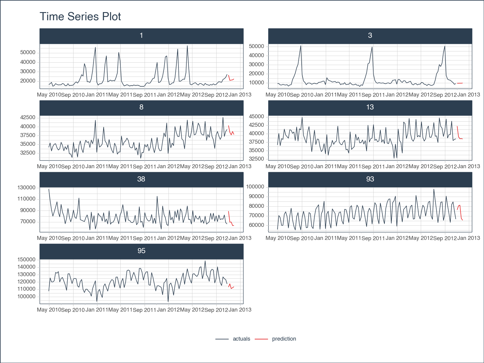
<Figure Size: (800 x 600)>

Our weekly sales forecasts exhibit a noticeable alignment with historical trends, indicating that our models are effectively capturing essential data signals. It’s worth noting that with some additional feature engineering, we have the potential to further enhance the model’s performance.

Here are some additional techniques that can be explored to elevate its performance:

1. Experiment with the incorporation of various lags using the versatile tk.augment_lags() function.
2. Enhance the model’s capabilities by introducing additional rolling calculations through tk.augment_rolling().
3. Consider incorporating cyclic features by utilizing tk.augment_fourier().
4. Try different models and build a robust cross-validation strategy for model selection.

These strategies hold promise for refining the model’s accuracy and predictive power

3 Conclusion

This exemplifies the remarkable capabilities of pytimetk in aiding Data Scientists in conducting comprehensive time series analysis for demand forecasting. Throughout this process, we employed various pytimetk functions and techniques to enhance our analytical approach:

• We harnessed the power of tk.augment_time_signature() to generate a plethora of date features, enriching our dataset.
• The feature engineering functions tk.augment_lags() and tk.augment_rolling() from pytimetk played a pivotal role in our analysis, enabling us to create lag-based features and rolling calculations.
• Utilizing tk.future_frame(), we constructed our prediction set
• To gain valuable insights into our final model’s performance, we leveraged tk.plot_timeseries() to visualize our results.

These pytimetk features provide incredibly powerful techniques with a very easy strcuture and minimal code. They were indispensable in crafting a high-quality sales forecast, seamlessly integrated with sklearn.

4 More Coming Soon…

We are in the early stages of development. But it’s obvious the potential for pytimetk now in Python. 🐍

• Please ⭐ us on GitHub (it takes 2-seconds and means a lot).
• To make requests, please see our Project Roadmap GH Issue #2. You can make requests there.
• Want to contribute? See our contributing guide here.