Speed Comparisons

How this guide benefits you

This guide covers speed and performance comparisons using the polars backend.

Beginning in version 0.2.0 of pytimetk, we introduced new polars engines to many of our functions. This is aimed at leveraging the speed benefits of polars without requiring you (the user) to learn a new data manipulation framework.

1 Pytimetk Speed Result Summary

It’s typical to see 2X to 15X speedups just by using the polars engine. Speedups of 500X to 3500X are possible by using efficient functions (e.g. staying away from lambdas).

Features/Properties	polars	pandas
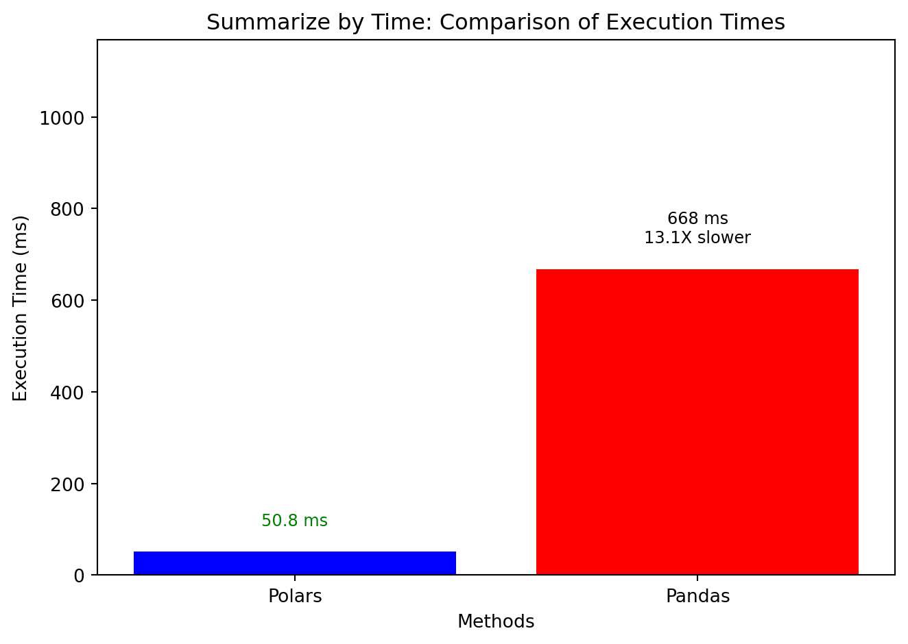
`summarize_by_time()`	🚀 13X Faster	🐢 Standard
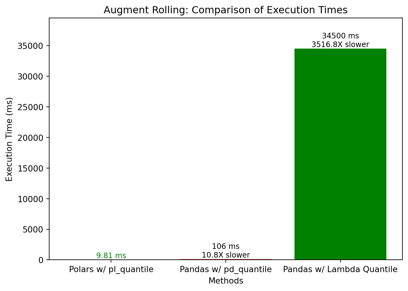
`augment_rolling()`	🚀 10X to 3500X Faster	🐢 Standard
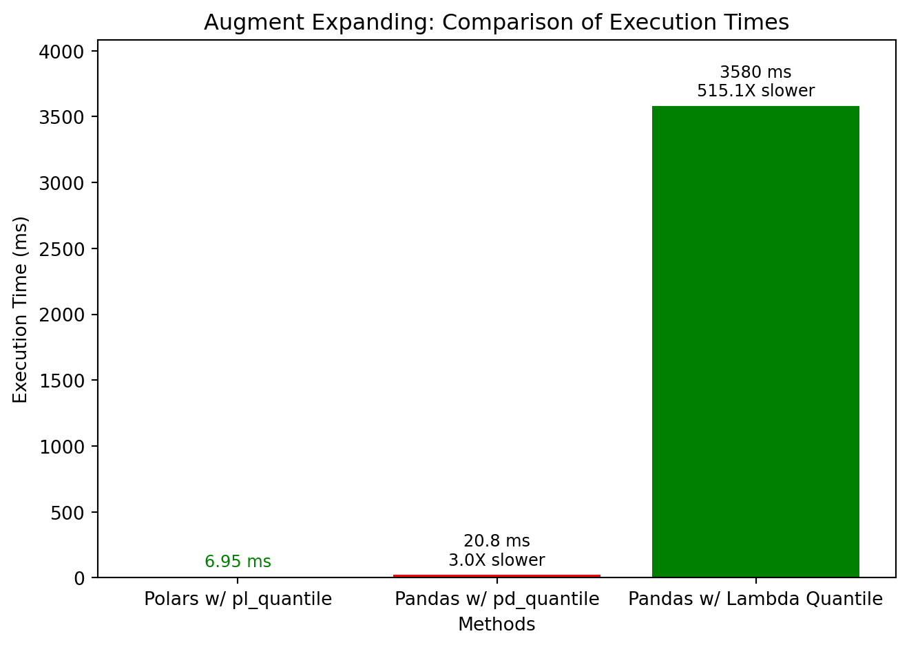
`augment_expanding()`	🚀 3X to 500X Faster	🐢 Standard
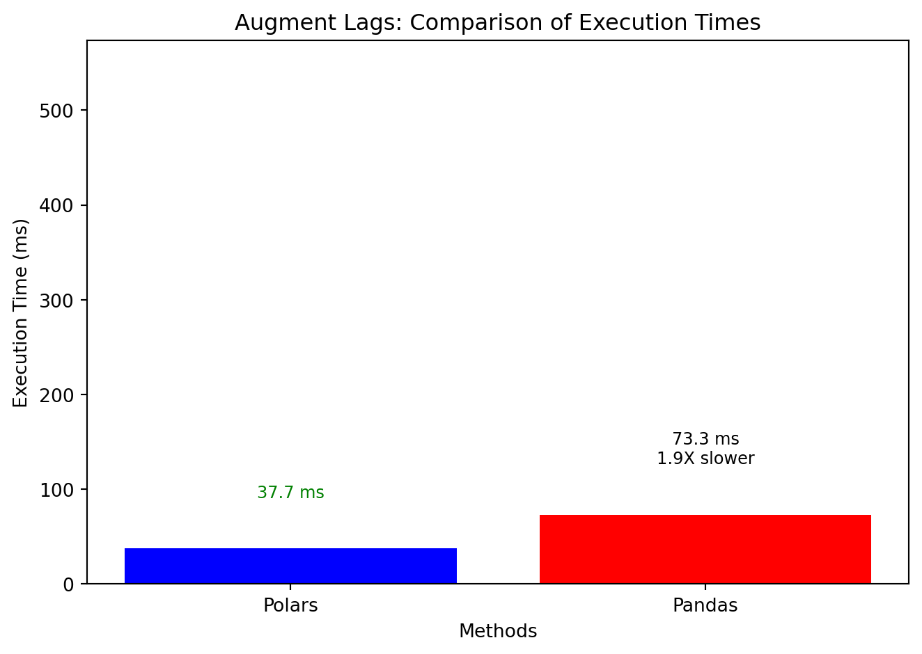
`augment_lags()`	🚀 2X to 20X Faster	🐢 Standard

2 About Performance

In time series, data is often large (<100M Rows), and contains many groups. Bbecause of this, computational efficiency is paramount. Beginning in pytimetk 0.2.0 we began introducing a new, polars backend to help improve the speed.

2.1 Key benefits:

You can get between 2X and 500X speed boost on many common time series operations
You don’t need to know how to use polars to gain massive speed boosts
Simply turn engine = 'polars' to get the speed boost.

2.2 What affects speed?

Many factors can affect speed. Things that are known to slow performance down:

Using non-optimized “lambda” functions. Lambda Functions are created at runtime. This process is flexible but extremely inefficient. Where possible use “built-in” or “configurable” functions instead.
Not using polars. Polars is built on top of Rust, which is a low-level language known for performance and optimized for speed. Using polars usually speeds up computation versus Pandas.

3 Speed Tests and Conclusions

Load the packages and datasets needed to replicate the speed tests (Click to Expand):

Code

# Libraries
import pytimetk as tk
import pandas as pd
import numpy as np
import matplotlib.pyplot as plt

from pytimetk.utils.polars_helpers import pl_quantile
from pytimetk.utils.pandas_helpers import pd_quantile

# Datasets
expedia_df = tk.load_dataset("expedia", parse_dates = ['date_time'])
m4_daily_df = tk.load_dataset("m4_daily", parse_dates = ['date'])
stocks_daily_df = tk.load_dataset('stocks_daily', parse_dates=['date'])

# Plotting utility
def make_time_comparison_plot(title, methods, times, height_spacer=500):
    """
    Create a bar chart comparing execution times of different methods.
    
    Args:
    - title (str): Title for the plot.
    - methods (list of str): Names of the methods being compared.
    - times (list of float): Execution times corresponding to the methods.
    - height_spacer (int, optional): Additional space above the tallest bar. Defaults to 5000.
    
    Returns:
    - None. Displays the plot.
    """
    
    # Calculate how many times slower each method is relative to the fastest method
    min_time = min(times)
    times_slower = [time / min_time for time in times]

    # Create the bar chart
    bars = plt.bar(methods, times, color=['blue', 'red', 'green', 'orange'])

    # Add title and labels
    plt.title(f'{title}: Comparison of Execution Times')
    plt.ylabel('Execution Time (ms)')
    plt.xlabel('Methods')

    # Display the execution times and how many times slower on top of the bars
    for bar, v, multiplier in zip(bars, times, times_slower):
        height = bar.get_height()
        plt.text(bar.get_x() + bar.get_width() / 2, height + 50, 
                 f"{v} ms\n{multiplier:.1f}X slower" if multiplier != 1 else f"{v} ms", 
                 ha='center', va='bottom', fontsize=9, 
                 color='black' if multiplier != 1 else 'green')

    # Adjust y-axis limit to make sure all labels fit
    plt.ylim(0, max(times) + height_spacer)

    # Display the plot
    plt.tight_layout()
    return plt

4 Feature Engineering Performance Comparisons

This section includes performance comparisons are common Time Series Feature Engineering tasks.

4.1 Summarize By Time `summarize_by_time()`

Polars is 13.1X faster than Pandas

Polars
Pandas

Code

%%timeit -n 10

df_pytimetk = expedia_df[['site_name', 'date_time', 'cnt', 'is_booking']] \
    .groupby('site_name') \
    .summarize_by_time(
        date_column = 'date_time',
        value_column = ['cnt', 'is_booking'],
        freq = 'W',
        agg_func = ['sum', 'count'],
        engine = 'polars'
    )

# 50.8 ms ± 2.45 ms per loop (mean ± std. dev. of 7 runs, 10 loops each)

Code

%%timeit -n 10

df_pytimetk = expedia_df[['site_name', 'date_time', 'cnt', 'is_booking']] \
    .groupby('site_name') \
    .summarize_by_time(
        date_column = 'date_time',
        value_column = ['cnt', 'is_booking'],
        freq = 'W',
        agg_func = ['sum', 'count'],
        engine = 'pandas'
    )

# 668 ms ± 16.5 ms per loop (mean ± std. dev. of 7 runs, 10 loops each)

4.2 Rolling Calculations `augment_rolling()`

Polars is 10.8X faster than Pandas
Polars is 3,517X faster than Pandas with Lambdas

Uses pl_quantile() configurable function.

Code

%%timeit

expanded_df = (
    m4_daily_df
        .groupby('id')
        .augment_rolling(
            date_column = 'date', 
            value_column = 'value', 
            window = (1,10),
            window_func = [
                'mean',  # Built-in mean function
                'std',   # Built-in std function
                ('quantile_75', pl_quantile(quantile=0.75)),  # Configurable with all parameters found in polars.Expr.rolling_quantile
            ],
            min_periods = 1,
            engine = 'polars',
        )
)
# 9.81 ms ± 116 µs per loop (mean ± std. dev. of 7 runs, 100 loops each)

Uses pd_quantile() configurable function.

Code

%%timeit

expanded_df = (
    m4_daily_df
        .groupby('id')
        .augment_rolling(
            date_column = 'date', 
            value_column = 'value', 
            window = (1,10),
            window_func = [
                'mean',  # Built-in mean function
                'std',   # Built-in standard deviation function,
                # ('quantile_75', lambda x: pd.Series(x).quantile(0.75)),  # Custom quantile function
                ('quantile_75', pd_quantile(q=0.75))
            ],
            min_periods = 1,
            engine = 'pandas',  # Utilize pandas for the underlying computations
            show_progress = False,
        )
)

# 106 ms ± 2.38 ms per loop (mean ± std. dev. of 7 runs, 10 loops each)

Uses lambda x: pd.Series(x).quantile(0.75). Lambda functions are extremely inefficient.

Code

%%timeit

expanded_df = (
    m4_daily_df
        .groupby('id')
        .augment_rolling(
            date_column = 'date', 
            value_column = 'value', 
            window = (1,10),
            window_func = [
                'mean',  # Built-in mean function
                'std',   # Built-in standard deviation function,
                ('quantile_75', lambda x: pd.Series(x).quantile(0.75)), # lambda slows things down
            ],
            min_periods = 1,
            engine = 'pandas',  
            show_progress = False,
        )
)

# 34.5 s ± 236 ms per loop (mean ± std. dev. of 7 runs, 1 loop each)

4.3 Augment Expanding `augment_expanding()`

Polars is 3X faster than Pandas with built-in and configurable functions
Polars is 515X faster than Pandas with lambda functions

Uses pl_quantile() configurable function.

Code

%%timeit

expanded_df = (
    m4_daily_df
        .groupby('id')
        .augment_expanding(
            date_column = 'date', 
            value_column = 'value', 
            window_func = [
                'mean',  # Built-in mean function
                'std',   # Built-in std function
                ('quantile_75', pl_quantile(quantile=0.75)),  # Configurable with all parameters found in polars.Expr.rolling_quantile
            ],
            min_periods = 1,
            engine = 'polars',
        )
)
# 6.95 ms ± 163 µs per loop (mean ± std. dev. of 7 runs, 100 loops each)

Uses pd_quantile() configurable function.

Code

%%timeit

expanded_df = (
    m4_daily_df
        .groupby('id')
        .augment_expanding(
            date_column = 'date', 
            value_column = 'value', 
            window_func = [
                'mean',  # Built-in mean function
                'std',   # Built-in standard deviation function,
                # ('quantile_75', lambda x: pd.Series(x).quantile(0.75)),  # Custom quantile function
                ('quantile_75', pd_quantile(q=0.75))
            ],
            min_periods = 1,
            engine = 'pandas',  # Utilize pandas for the underlying computations
        )
)

# 20.8 ms ± 1.51 ms per loop (mean ± std. dev. of 7 runs, 10 loops each)

Uses lambda x: pd.Series(x).quantile(0.75). Lambda functions are extremely inefficient.

Code

%%timeit

expanded_df = (
    m4_daily_df
        .groupby('id')
        .augment_expanding(
            date_column = 'date', 
            value_column = 'value', 
            window_func = [
                'mean',  # Built-in mean function
                'std',   # Built-in standard deviation function,
                ('quantile_75', lambda x: pd.Series(x).quantile(0.75)), # lambda slows things down
            ],
            min_periods = 1,
            engine = 'pandas',  
        )
)

# 3.58 s ± 110 ms per loop (mean ± std. dev. of 7 runs, 1 loop each)

4.4 Augment Lags `augment_lags()`

Polars is 1.9X faster than Pandas
Speed improvement of Polars (vs Pandas) increases with number of lags

Polars
Pandas

Code

%%timeit -n 25

expanded_df = (
    m4_daily_df
        .groupby('id')
        .augment_lags(
            date_column = 'date', 
            value_column = 'value', 
            lags = (2,30),
            engine = 'polars',  
        )
)

# 37.7 ms ± 1.57 ms per loop (mean ± std. dev. of 7 runs, 25 loops each)

Code

%%timeit -n 25

expanded_df = (
    m4_daily_df
        .groupby('id')
        .augment_lags(
            date_column = 'date', 
            value_column = 'value', 
            lags = (2,30),
            engine = 'pandas',  
        )
)

# 73.3 ms ± 3.29 ms per loop (mean ± std. dev. of 7 runs, 25 loops each)

5 Finance and Techincal Trading Performance Comparisons

5.1 Chande Momentum Oscillator (CMO) `augment_cmo()`

Polars is 3.3X faster than Pandas
Speed improvement of Polars (vs Pandas) increases with number of CMO periods

Polars
Pandas

Code

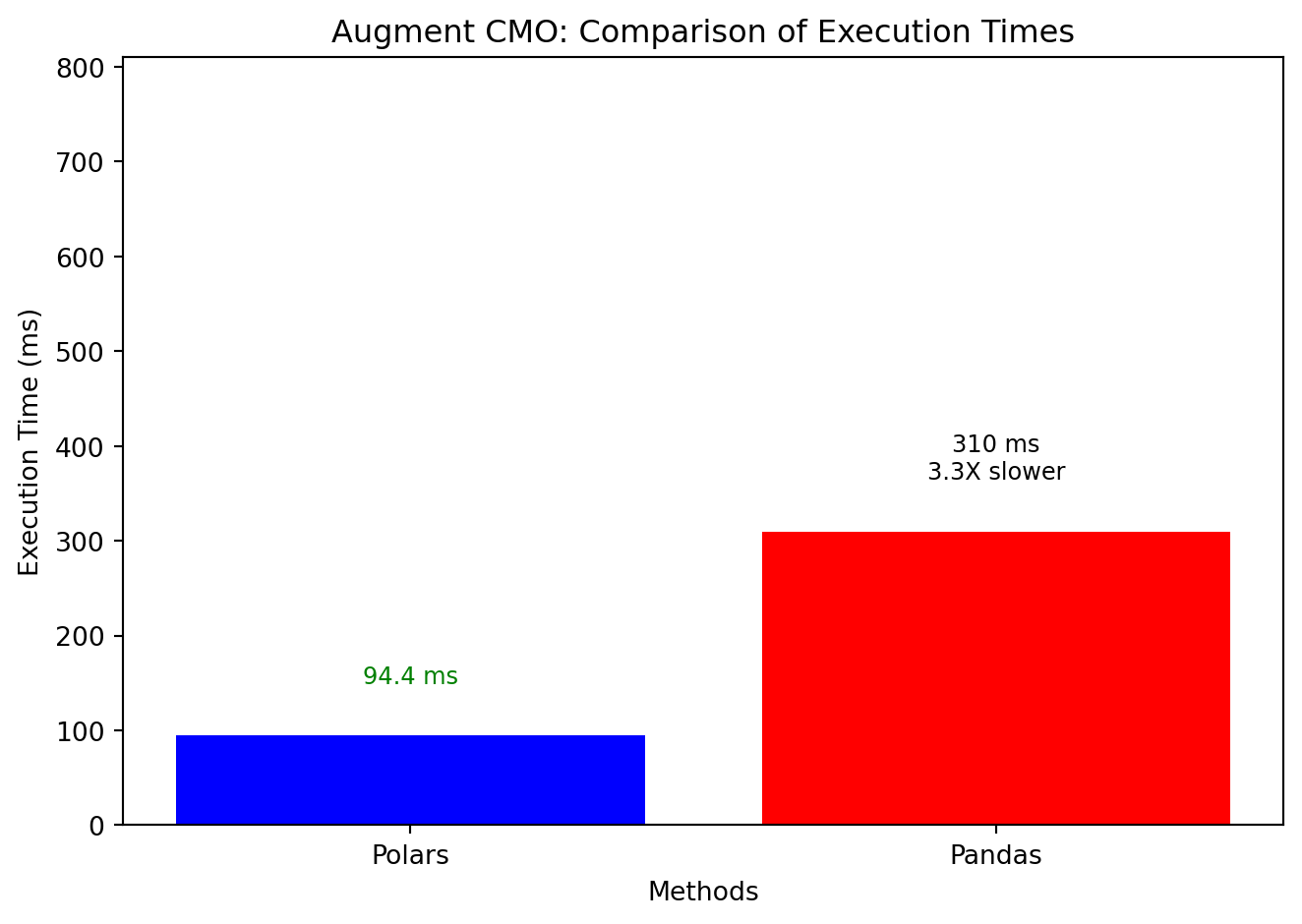
%%timeit -n 25

df = (
    stocks_daily_df
        .groupby('symbol')
        .augment_cmo(
            date_column = 'date', 
            value_column = 'adjusted', 
            periods = (5,30),
            engine = 'polars',  
        )
)

# 94.4 ms ± 3.24 ms per loop (mean ± std. dev. of 7 runs, 25 loops each)

Code

%%timeit -n 25

df = (
    stocks_daily_df
        .groupby('symbol')
        .augment_cmo(
            date_column = 'date', 
            value_column = 'adjusted', 
            periods = (5,30),
            engine = 'pandas',  
        )
)

# 73.3 ms ± 3.29 ms per loop (mean ± std. dev. of 7 runs, 25 loops each)

6 Conclusions

In general, when speed and performance is needed, which is quite often the case in large-scale time series databases (e.g. finance, customer analytics), the polars engine can be a substantial performance enhancer. Almost every function has experienced a performance increase with the new polars engine. We’ve seen many functions gain 10X increases and beyond.

7 More Coming Soon…

We are in the early stages of development. But it’s obvious the potential for pytimetk now in Python. 🐍

Please ⭐ us on GitHub (it takes 2-seconds and means a lot).
To make requests, please see our Project Roadmap GH Issue #2. You can make requests there.
Want to contribute? See our contributing guide here.

1 Pytimetk Speed Result Summary

2 About Performance

2.1 Key benefits:

2.2 What affects speed?

3 Speed Tests and Conclusions

4 Feature Engineering Performance Comparisons

4.1 Summarize By Time summarize_by_time()

4.2 Rolling Calculations augment_rolling()

4.3 Augment Expanding augment_expanding()

4.4 Augment Lags augment_lags()

5 Finance and Techincal Trading Performance Comparisons

5.1 Chande Momentum Oscillator (CMO) augment_cmo()

6 Conclusions

7 More Coming Soon…

4.1 Summarize By Time `summarize_by_time()`

4.2 Rolling Calculations `augment_rolling()`

4.3 Augment Expanding `augment_expanding()`

4.4 Augment Lags `augment_lags()`

5.1 Chande Momentum Oscillator (CMO) `augment_cmo()`