Sales Analysis

In this tutorial, we will use pytimetk and its powerful functions to perform a time series analysis on a dataset representing bike sales. Our goal is to understand the patterns in the data and forecast future sales. You will:

Examine ways to wrangle complex transactional data with tk.summarize_by_time
Discover how to visualize customer and product data with tk.plot_timeseries
Using tk.pad_by_time and tk.future_frame to prepare data for modeling
Learn how to add many important time series features with augment functions including tk.augment_timeseries_signature and tk.agument_lags
Integrate these techniques into a sales forecast with sklearn

1 Tutorial Setup

1.1 Load Packages.

If you do not have pytimetk installed, you can install by using

pip install pytimetk

or for the latest features and functionality, you can install the development version.

pip install git+https://github.com/business-science/pytimetk.git

Code

import pytimetk as tk
import pandas as pd
import numpy as np

from sklearn.ensemble import RandomForestRegressor
from sklearn.model_selection import train_test_split

1.2 Load & inspect dataset

To kick off our analysis, we’ll begin by importing essential libraries and accessing the ‘bike_sales’ dataset available within pytimetk’s suite of built-in datasets.

The Bike Sales dataset exemplifies what one might find in a CRM (Customer Relationship Management) system. CRM systems are pivotal for businesses, offering vital insights by tracking sales throughout the entire sales funnel. Such datasets are rich with transaction-level data, encompassing elements like order numbers, individual order lines, customer details, product information, and specific transaction data.

Transactional data, such as this, inherently holds the essential components for time series analysis:

Time Stamps
Associated Values
Distinct Groups or Categories

Given these attributes, the Bike Sales dataset emerges as an ideal candidate for analysis using pytimetk.

2 Exploratory Analysis

2.1 Initial Inspection with `tk.glimpse`

To get a preliminary understanding of our data, let’s utilize the tk.glimpse() function from pytimetk. This will provide us with a snapshot of the available fields, their respective data types, and a sneak peek into the data entries.

Code

df = tk.datasets.load_dataset('bike_sales_sample')
df['order_date'] = pd.to_datetime(df['order_date'])

df.glimpse()

<class 'pandas.core.frame.DataFrame'>: 2466 rows of 13 columns
order_id:        int64             [1, 1, 2, 2, 3, 3, 3, 3, 3, 4, 5, 5,  ...
order_line:      int64             [1, 2, 1, 2, 1, 2, 3, 4, 5, 1, 1, 2,  ...
order_date:      datetime64[ns]    [Timestamp('2011-01-07 00:00:00'), Ti ...
quantity:        int64             [1, 1, 1, 1, 1, 1, 1, 1, 1, 1, 1, 2,  ...
price:           int64             [6070, 5970, 2770, 5970, 10660, 3200, ...
total_price:     int64             [6070, 5970, 2770, 5970, 10660, 3200, ...
model:           object            ['Jekyll Carbon 2', 'Trigger Carbon 2 ...
category_1:      object            ['Mountain', 'Mountain', 'Mountain',  ...
category_2:      object            ['Over Mountain', 'Over Mountain', 'T ...
frame_material:  object            ['Carbon', 'Carbon', 'Aluminum', 'Car ...
bikeshop_name:   object            ['Ithaca Mountain Climbers', 'Ithaca  ...
city:            object            ['Ithaca', 'Ithaca', 'Kansas City', ' ...
state:           object            ['NY', 'NY', 'KS', 'KS', 'KY', 'KY',  ...

2.2 Data Exploration with `tk.summarize_by_time`

CRM data is often bustling with activity, reflecting the myriad of transactions happening daily. Due to this high volume, the data can sometimes seem overwhelming or noisy. To derive meaningful insights, it’s essential to aggregate this data over specific time intervals. This is where tk.summarize_by_time() comes into play.

The tk.summarize_by_time() function offers a streamlined approach to time-based data aggregation. By defining a desired frequency and an aggregation method, this function seamlessly organizes your data. The beauty of it is its versatility; from a broad array of built-in aggregation methods and frequencies to the flexibility of integrating a custom function, it caters to a range of requirements.

Getting to know tk.summarize_by_time()

Curious about the various options it provides?

Click here to see our Data Wrangling Guide
Use help(tk.summarize_by_time) to review additional helpful documentation. And explore the plethora of possibilities!

Getting Weekly Totals

We can quickly get totals by week with summarize_byt_time.

Code

weekly_totals = df.summarize_by_time(
    date_column  = 'order_date',
    value_column = 'total_price',
    agg_func     = ['sum'],
    freq         = 'W'
)

weekly_totals.head(10)

	order_date	total_price_sum
0	2011-01-09	12040
1	2011-01-16	151460
2	2011-01-23	143850
3	2011-01-30	175665
4	2011-02-06	105210
5	2011-02-13	250390
6	2011-02-20	410595
7	2011-02-27	254045
8	2011-03-06	308420
9	2011-03-13	45450

Get Weekly Totals by Group (Category 2)

To better understand your data, you might want to add groups to this summary. We can include a groupby before the summarize_by_time and then aggregate our data.

Code

 sales_by_week = df \
    .groupby('category_2') \
    .summarize_by_time(
        date_column = 'order_date',
        value_column = 'total_price',
        agg_func = ['sum'],
        freq = 'W'
    )

sales_by_week.head(10)

	category_2	order_date	total_price_sum
0	Cross Country Race	2011-01-16	61750
1	Cross Country Race	2011-01-23	25050
2	Cross Country Race	2011-01-30	56860
3	Cross Country Race	2011-02-06	8740
4	Cross Country Race	2011-02-13	78070
5	Cross Country Race	2011-02-20	115010
6	Cross Country Race	2011-02-27	64290
7	Cross Country Race	2011-03-06	95070
8	Cross Country Race	2011-03-13	3200
9	Cross Country Race	2011-03-20	21170

Long vs Wide Format

This long format can make it a little hard to compare the different group values visually, so instead of long-format you might want to pivot wide to view the data.

Code

sales_by_week_wide = df \
    .groupby('category_2') \
    .summarize_by_time(
        date_column = 'order_date',
        value_column = 'total_price',
        agg_func = ['sum'],
        freq = 'W',
        wide_format = True
    )

sales_by_week_wide.head(10)

	order_date	total_price_sum_Cross Country Race	total_price_sum_Cyclocross	total_price_sum_Elite Road	total_price_sum_Endurance Road	total_price_sum_Fat Bike	total_price_sum_Over Mountain	total_price_sum_Sport	total_price_sum_Trail	total_price_sum_Triathalon
0	2011-01-09	0.0	0.0	0.0	0.0	0.0	12040.0	0.0	0.0	0.0
1	2011-01-16	61750.0	1960.0	49540.0	11110.0	0.0	9170.0	4030.0	7450.0	6450.0
2	2011-01-23	25050.0	3500.0	51330.0	47930.0	0.0	3840.0	0.0	0.0	12200.0
3	2011-01-30	56860.0	2450.0	43895.0	24160.0	0.0	10880.0	3720.0	26700.0	7000.0
4	2011-02-06	8740.0	7000.0	35640.0	22680.0	3730.0	14270.0	980.0	10220.0	1950.0
5	2011-02-13	78070.0	0.0	83780.0	24820.0	2130.0	17160.0	6810.0	17120.0	20500.0
6	2011-02-20	115010.0	7910.0	79770.0	27650.0	26100.0	37830.0	10925.0	96250.0	9150.0
7	2011-02-27	64290.0	6650.0	86900.0	31900.0	5860.0	22070.0	6165.0	16410.0	13800.0
8	2011-03-06	95070.0	2450.0	31990.0	47660.0	5860.0	82060.0	9340.0	26790.0	7200.0
9	2011-03-13	3200.0	4200.0	23110.0	7260.0	0.0	5970.0	1710.0	0.0	0.0

You can now observe the total sales for each product side by side. This streamlined view facilitates easy comparison between product sales.

2.3 Visualize your time series data with `tk.plot_timeseries`

You can now visualize the summarized data to gain a clearer insight into the prevailing trends.

Plotly
Plotnine

Code

sales_by_week \
    .groupby('category_2') \
    .plot_timeseries(
        date_column = 'order_date',  
        value_column = 'total_price_sum',
        title = 'Bike Sales by Category',
        facet_ncol = 2,
        facet_scales = "free",
        y_intercept_color = tk.palette_timetk()['steel_blue'],
        width = 1000,
        height = 800,
        y_lab = 'Total Sales', 
        engine = 'plotly'
    )

Code

sales_by_week \
    .groupby('category_2') \
    .plot_timeseries(
        date_column = 'order_date',  
        value_column = 'total_price_sum',
        title = 'Bike Sales by Category',
        facet_ncol = 2,
        facet_scales = "free",
        y_intercept_color = tk.palette_timetk()['steel_blue'],
        width = 1000,
        height = 800,
        y_lab = 'Total Sales', 
        engine = 'plotnine'
    )

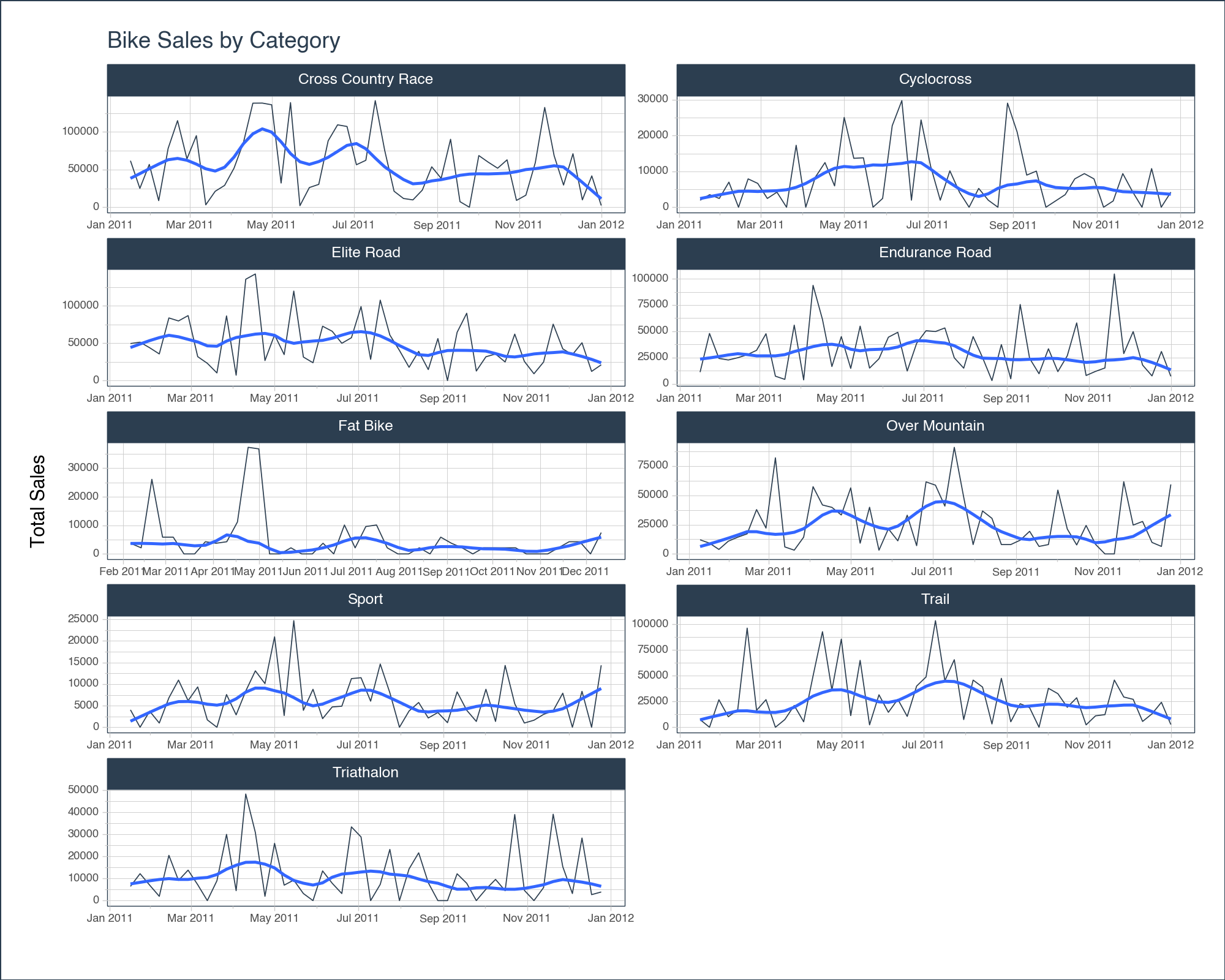
<Figure Size: (1000 x 800)>

The graph showcases a pronounced uptick in sales for most of the different bike products during the summer. It’s a natural trend, aligning with our understanding that people gravitate towards biking during the balmy summer days. Conversely, as the chill of winter sets in at the year’s start and end, we observe a corresponding dip in sales.

It’s worth highlighting the elegance of the plot_timeseries function. Beyond just plotting raw data, it introduces a smoother, accentuating underlying trends and making them more discernible. This enhancement ensures we can effortlessly capture and comprehend the cyclical nature of bike sales throughout the year.

3 Create a Product Forecast Model

Forecasting future sales for bikes requires meticulous data preparation, and pytimetk streamlines this process for us. When crafting a Machine Learning model tailored for time series analysis, there are several pivotal steps to follow:

Time Padding for Comprehensive Historical Data: It’s essential to ensure that our data captures every week, even those that witnessed zero sales. This padding becomes especially pertinent when integrating time series features, like lags.
Crafting the Future Frame: This step involves setting up a structure that accommodates the test data features, which will eventually be fed into our prediction function.
Infusing Time Series Lag Features: These features are critical for capturing patterns in time series data, and they need to be integrated into our future frame.
Feature / Date Augmentation: This step can involve adding contextual features that might influence sales, such as date features, holidays, promotional events, etc.
Model Training: Once the data is prepped, it’s time to train our Machine Learning model, refining it to understand historical patterns and predict future trends.
Making Predictions: After training, the model is ready to forecast sales for future periods based on the features of the new data.

3.1 Making irregular data regular with `tk.pad_by_time`

Kicking off our journey, we’ll utilize pytimetk’s tk.pad_by_time() function. For this, grouping by the ‘category_1’ variable is recommended. Moreover, it’s prudent to establish a definitive end date. This ensures that all groups are equipped with training data up to the most recent date, accommodating scenarios where certain categories might have seen no sales in the final training week. By doing so, we create a representative observation for every group, capturing the nuances of each category’s sales pattern.

Code

sales_padded = sales_by_week \
    .groupby('category_2') \
    .pad_by_time(
        date_column = 'order_date',
        freq        = 'W',
        end_date    = sales_by_week.order_date.max()
    )
sales_padded

	category_2	order_date	total_price_sum
0	Cross Country Race	2011-01-09	NaN
1	Cross Country Race	2011-01-16	61750.0
2	Cross Country Race	2011-01-23	25050.0
3	Cross Country Race	2011-01-30	56860.0
4	Cross Country Race	2011-02-06	8740.0
...	...	...	...
463	Triathalon	2011-12-04	3200.0
464	Triathalon	2011-12-11	28350.0
465	Triathalon	2011-12-18	2700.0
466	Triathalon	2011-12-25	3900.0
467	Triathalon	2012-01-01	NaN

468 rows × 3 columns

3.2 Making Future Dates Easier with `tk.future_frame`

Moving on, let’s set up the future frame, which will serve as our test dataset. To achieve this, employ the tk.future_frame() method. This function allows for the specification of a grouping column and a forecast horizon.

Upon invoking tk.future_frame(), you’ll observe that placeholders (null values) are added for each group, extending 12 weeks into the future.

Code

df_with_futureframe = sales_padded \
    .groupby('category_2') \
    .future_frame(
        date_column = 'order_date',
        length_out  = 12
    )
df_with_futureframe

	category_2	order_date	total_price_sum
0	Cross Country Race	2011-01-09	NaN
1	Cross Country Race	2011-01-16	61750.0
2	Cross Country Race	2011-01-23	25050.0
3	Cross Country Race	2011-01-30	56860.0
4	Cross Country Race	2011-02-06	8740.0
...	...	...	...
571	Triathalon	2012-02-26	NaN
572	Triathalon	2012-03-04	NaN
573	Triathalon	2012-03-11	NaN
574	Triathalon	2012-03-18	NaN
575	Triathalon	2012-03-25	NaN

576 rows × 3 columns

3.3 Lag Values with `tk.augment_lags`

Crafting features from time series data can be intricate, but thanks to the suite of feature engineering tools in pytimetk, the process is streamlined and intuitive.

In this guide, we’ll focus on the basics: introducing a few lag variables and incorporating some date-related features.

Firstly, let’s dive into creating lag features.

Given our forecasting objective of a 12-week horizon, to ensure we have lag data available for every future point, we should utilize a lag of 12 or more. The beauty of the toolkit is that it supports the addition of multiple lags simultaneously.

Lag features play a pivotal role in machine learning for time series. Often, recent data offers valuable insights into future trends. To capture this recency effect, it’s crucial to integrate lag values. For this purpose, tk.augment_lags() comes in handy.

Code

df_with_lags = df_with_futureframe \
    .groupby('category_2') \
    .augment_lags(
        date_column  = 'order_date',
        value_column = 'total_price_sum',
        lags         = [12,24]

    )
df_with_lags.head(25)

	category_2	order_date	total_price_sum	total_price_sum_lag_12	total_price_sum_lag_24
0	Cross Country Race	2011-01-09	NaN	NaN	NaN
1	Cross Country Race	2011-01-16	61750.0	NaN	NaN
2	Cross Country Race	2011-01-23	25050.0	NaN	NaN
3	Cross Country Race	2011-01-30	56860.0	NaN	NaN
4	Cross Country Race	2011-02-06	8740.0	NaN	NaN
5	Cross Country Race	2011-02-13	78070.0	NaN	NaN
6	Cross Country Race	2011-02-20	115010.0	NaN	NaN
7	Cross Country Race	2011-02-27	64290.0	NaN	NaN
8	Cross Country Race	2011-03-06	95070.0	NaN	NaN
9	Cross Country Race	2011-03-13	3200.0	NaN	NaN
10	Cross Country Race	2011-03-20	21170.0	NaN	NaN
11	Cross Country Race	2011-03-27	28990.0	NaN	NaN
12	Cross Country Race	2011-04-03	51860.0	NaN	NaN
13	Cross Country Race	2011-04-10	85910.0	61750.0	NaN
14	Cross Country Race	2011-04-17	138230.0	25050.0	NaN
15	Cross Country Race	2011-04-24	138350.0	56860.0	NaN
16	Cross Country Race	2011-05-01	136090.0	8740.0	NaN
17	Cross Country Race	2011-05-08	32110.0	78070.0	NaN
18	Cross Country Race	2011-05-15	139010.0	115010.0	NaN
19	Cross Country Race	2011-05-22	2060.0	64290.0	NaN
20	Cross Country Race	2011-05-29	26130.0	95070.0	NaN
21	Cross Country Race	2011-06-05	30360.0	3200.0	NaN
22	Cross Country Race	2011-06-12	88280.0	21170.0	NaN
23	Cross Country Race	2011-06-19	109470.0	28990.0	NaN
24	Cross Country Race	2011-06-26	107280.0	51860.0	NaN

Observe that lag values of 12 and 24 introduce missing entries at the dataset’s outset. This occurs because there isn’t available data from 12 or 24 weeks prior. To address these gaps, you can adopt one of two strategies:

Discard the Affected Rows: This is a recommended approach if your dataset is sufficiently large. Removing a few initial rows might not significantly impact the training process.
Backfill Missing Values: In situations with limited data, you might consider backfilling these nulls using the first available values from lag 12 and 24. However, the appropriateness of this technique hinges on your specific context and objectives.

For the scope of this tutorial, we’ll opt to remove these rows. However, it’s worth pointing out that our dataset is quite small with limited historical data, so this might impact our model.

Code

lag_columns = [col for col in df_with_lags.columns if 'lag' in col]
df_no_nas = df_with_lags \
    .dropna(subset=lag_columns, inplace=False)

df_no_nas.head()

	category_2	order_date	total_price_sum	total_price_sum_lag_12	total_price_sum_lag_24
25	Cross Country Race	2011-07-03	56430.0	85910.0	61750.0
26	Cross Country Race	2011-07-10	62320.0	138230.0	25050.0
27	Cross Country Race	2011-07-17	141620.0	138350.0	56860.0
28	Cross Country Race	2011-07-24	75720.0	136090.0	8740.0
29	Cross Country Race	2011-07-31	21240.0	32110.0	78070.0

3.4 Date Features with `tk.augment_timeseries_signature`

Now, let’s enrich our dataset with date-related features.

With the function tk.augment_timeseries_signature(), you can effortlessly append 29 date attributes to a timestamp. Given that our dataset captures weekly intervals, certain attributes like ‘hour’ may not be pertinent. Thus, it’s prudent to refine our columns, retaining only those that truly matter to our analysis.

Code

df_with_datefeatures = df_no_nas \
    .augment_timeseries_signature(date_column='order_date')

df_with_datefeatures.head(10)

	category_2	order_date	total_price_sum	total_price_sum_lag_12	total_price_sum_lag_24	order_date_index_num	order_date_year	order_date_year_iso	...	order_date_mday	order_date_qday	order_date_yday	order_date_weekend	order_date_am_pm
25	Cross Country Race	2011-07-03	56430.0	85910.0	61750.0	1309651200	2011	2011	...	3	3	184	1	am
26	Cross Country Race	2011-07-10	62320.0	138230.0	25050.0	1310256000	2011	2011	...	10	10	191	1	am
27	Cross Country Race	2011-07-17	141620.0	138350.0	56860.0	1310860800	2011	2011	...	17	17	198	1	am
28	Cross Country Race	2011-07-24	75720.0	136090.0	8740.0	1311465600	2011	2011	...	24	24	205	1	am
29	Cross Country Race	2011-07-31	21240.0	32110.0	78070.0	1312070400	2011	2011	...	31	31	212	1	am
30	Cross Country Race	2011-08-07	11620.0	139010.0	115010.0	1312675200	2011	2011	...	7	38	219	1	am
31	Cross Country Race	2011-08-14	9730.0	2060.0	64290.0	1313280000	2011	2011	...	14	45	226	1	am
32	Cross Country Race	2011-08-21	22780.0	26130.0	95070.0	1313884800	2011	2011	...	21	52	233	1	am
33	Cross Country Race	2011-08-28	53680.0	30360.0	3200.0	1314489600	2011	2011	...	28	59	240	1	am
34	Cross Country Race	2011-09-04	38360.0	88280.0	21170.0	1315094400	2011	2011	...	4	66	247	1	am

10 rows × 34 columns

We can quickly get a sense of what features were just created using tk.glimpse.

Code

df_with_datefeatures.glimpse()

<class 'pandas.core.frame.DataFrame'>: 341 rows of 34 columns
category_2:               object            ['Cross Country Race', 'Cros ...
order_date:               datetime64[ns]    [Timestamp('2011-07-03 00:00 ...
total_price_sum:          float64           [56430.0, 62320.0, 141620.0, ...
total_price_sum_lag_12:   float64           [85910.0, 138230.0, 138350.0 ...
total_price_sum_lag_24:   float64           [61750.0, 25050.0, 56860.0,  ...
order_date_index_num:     int64             [1309651200, 1310256000, 131 ...
order_date_year:          int64             [2011, 2011, 2011, 2011, 201 ...
order_date_year_iso:      UInt32            [2011, 2011, 2011, 2011, 201 ...
order_date_yearstart:     uint8             [0, 0, 0, 0, 0, 0, 0, 0, 0,  ...
order_date_yearend:       uint8             [0, 0, 0, 0, 0, 0, 0, 0, 0,  ...
order_date_leapyear:      uint8             [0, 0, 0, 0, 0, 0, 0, 0, 0,  ...
order_date_half:          int64             [2, 2, 2, 2, 2, 2, 2, 2, 2,  ...
order_date_quarter:       int64             [3, 3, 3, 3, 3, 3, 3, 3, 3,  ...
order_date_quarteryear:   object            ['2011Q3', '2011Q3', '2011Q3 ...
order_date_quarterstart:  uint8             [0, 0, 0, 0, 0, 0, 0, 0, 0,  ...
order_date_quarterend:    uint8             [0, 0, 0, 0, 0, 0, 0, 0, 0,  ...
order_date_month:         int64             [7, 7, 7, 7, 7, 8, 8, 8, 8,  ...
order_date_month_lbl:     object            ['July', 'July', 'July', 'Ju ...
order_date_monthstart:    uint8             [0, 0, 0, 0, 0, 0, 0, 0, 0,  ...
order_date_monthend:      uint8             [0, 0, 0, 0, 1, 0, 0, 0, 0,  ...
order_date_yweek:         UInt32            [26, 27, 28, 29, 30, 31, 32, ...
order_date_mweek:         int64             [1, 2, 3, 4, 5, 1, 2, 3, 4,  ...
order_date_wday:          int64             [7, 7, 7, 7, 7, 7, 7, 7, 7,  ...
order_date_wday_lbl:      object            ['Sunday', 'Sunday', 'Sunday ...
order_date_mday:          int64             [3, 10, 17, 24, 31, 7, 14, 2 ...
order_date_qday:          int64             [3, 10, 17, 24, 31, 38, 45,  ...
order_date_yday:          int64             [184, 191, 198, 205, 212, 21 ...
order_date_weekend:       int64             [1, 1, 1, 1, 1, 1, 1, 1, 1,  ...
order_date_hour:          int64             [0, 0, 0, 0, 0, 0, 0, 0, 0,  ...
order_date_minute:        int64             [0, 0, 0, 0, 0, 0, 0, 0, 0,  ...
order_date_second:        int64             [0, 0, 0, 0, 0, 0, 0, 0, 0,  ...
order_date_msecond:       int64             [0, 0, 0, 0, 0, 0, 0, 0, 0,  ...
order_date_nsecond:       int64             [0, 0, 0, 0, 0, 0, 0, 0, 0,  ...
order_date_am_pm:         object            ['am', 'am', 'am', 'am', 'am ...

Let’s subset to just a few of the relevant date features. Let’s use tk.glimpse again.

Code

df_with_datefeatures_narrom = df_with_datefeatures[[
    'order_date', 
    'category_2', 
    'total_price_sum',
    'total_price_sum_lag_12',
    'total_price_sum_lag_24',
    'order_date_year',  
    'order_date_half', 
    'order_date_quarter',      
    'order_date_month',
    'order_date_yweek'
]]

df_with_datefeatures_narrom.glimpse()

<class 'pandas.core.frame.DataFrame'>: 341 rows of 10 columns
order_date:              datetime64[ns]    [Timestamp('2011-07-03 00:00: ...
category_2:              object            ['Cross Country Race', 'Cross ...
total_price_sum:         float64           [56430.0, 62320.0, 141620.0,  ...
total_price_sum_lag_12:  float64           [85910.0, 138230.0, 138350.0, ...
total_price_sum_lag_24:  float64           [61750.0, 25050.0, 56860.0, 8 ...
order_date_year:         int64             [2011, 2011, 2011, 2011, 2011 ...
order_date_half:         int64             [2, 2, 2, 2, 2, 2, 2, 2, 2, 2 ...
order_date_quarter:      int64             [3, 3, 3, 3, 3, 3, 3, 3, 3, 3 ...
order_date_month:        int64             [7, 7, 7, 7, 7, 8, 8, 8, 8, 9 ...
order_date_yweek:        UInt32            [26, 27, 28, 29, 30, 31, 32,  ...

One-Hot Encoding

The final phase in our feature engineering journey is one-hot encoding our categorical variables. While certain machine learning models like CatBoost can natively handle categorical data, many cannot. Enter one-hot encoding, a technique that transforms each category within a column into its separate column, marking its presence with a ‘1’ or absence with a ‘0’.

For this transformation, the handy pd.get_dummies() function from pandas comes to the rescue.

Code

df_encoded = pd.get_dummies(df_with_datefeatures_narrom, columns=['category_2'])

df_encoded.glimpse()

<class 'pandas.core.frame.DataFrame'>: 341 rows of 18 columns
order_date:                     datetime64[ns]    [Timestamp('2011-07-03 ...
total_price_sum:                float64           [56430.0, 62320.0, 141 ...
total_price_sum_lag_12:         float64           [85910.0, 138230.0, 13 ...
total_price_sum_lag_24:         float64           [61750.0, 25050.0, 568 ...
order_date_year:                int64             [2011, 2011, 2011, 201 ...
order_date_half:                int64             [2, 2, 2, 2, 2, 2, 2,  ...
order_date_quarter:             int64             [3, 3, 3, 3, 3, 3, 3,  ...
order_date_month:               int64             [7, 7, 7, 7, 7, 8, 8,  ...
order_date_yweek:               UInt32            [26, 27, 28, 29, 30, 3 ...
category_2_Cross Country Race:  uint8             [1, 1, 1, 1, 1, 1, 1,  ...
category_2_Cyclocross:          uint8             [0, 0, 0, 0, 0, 0, 0,  ...
category_2_Elite Road:          uint8             [0, 0, 0, 0, 0, 0, 0,  ...
category_2_Endurance Road:      uint8             [0, 0, 0, 0, 0, 0, 0,  ...
category_2_Fat Bike:            uint8             [0, 0, 0, 0, 0, 0, 0,  ...
category_2_Over Mountain:       uint8             [0, 0, 0, 0, 0, 0, 0,  ...
category_2_Sport:               uint8             [0, 0, 0, 0, 0, 0, 0,  ...
category_2_Trail:               uint8             [0, 0, 0, 0, 0, 0, 0,  ...
category_2_Triathalon:          uint8             [0, 0, 0, 0, 0, 0, 0,  ...

Training and Future Feature Sets

Pytimetk offers an extensive array of feature engineering tools and augmentation functions, giving you a broad spectrum of possibilities. However, for the purposes of this tutorial, let’s shift our focus to modeling.

Let’s proceed by segmenting our dataframe into training and future sets.

Code

future = df_encoded[df_encoded.total_price_sum.isnull()]
train = df_encoded[df_encoded.total_price_sum.notnull()]

Let’s focus on the columns essential for training. You’ll observe that we’ve excluded the ‘order_date’ column. This is because numerous machine learning models struggle with date data types. This is precisely why we utilized the tk.augment_timeseries_signature earlier—to transform date features into a format that’s compatible with ML models.

We can quickly see what features we have available with tk.glimpse().

Code

train.glimpse()

<class 'pandas.core.frame.DataFrame'>: 233 rows of 18 columns
order_date:                     datetime64[ns]    [Timestamp('2011-07-03 ...
total_price_sum:                float64           [56430.0, 62320.0, 141 ...
total_price_sum_lag_12:         float64           [85910.0, 138230.0, 13 ...
total_price_sum_lag_24:         float64           [61750.0, 25050.0, 568 ...
order_date_year:                int64             [2011, 2011, 2011, 201 ...
order_date_half:                int64             [2, 2, 2, 2, 2, 2, 2,  ...
order_date_quarter:             int64             [3, 3, 3, 3, 3, 3, 3,  ...
order_date_month:               int64             [7, 7, 7, 7, 7, 8, 8,  ...
order_date_yweek:               UInt32            [26, 27, 28, 29, 30, 3 ...
category_2_Cross Country Race:  uint8             [1, 1, 1, 1, 1, 1, 1,  ...
category_2_Cyclocross:          uint8             [0, 0, 0, 0, 0, 0, 0,  ...
category_2_Elite Road:          uint8             [0, 0, 0, 0, 0, 0, 0,  ...
category_2_Endurance Road:      uint8             [0, 0, 0, 0, 0, 0, 0,  ...
category_2_Fat Bike:            uint8             [0, 0, 0, 0, 0, 0, 0,  ...
category_2_Over Mountain:       uint8             [0, 0, 0, 0, 0, 0, 0,  ...
category_2_Sport:               uint8             [0, 0, 0, 0, 0, 0, 0,  ...
category_2_Trail:               uint8             [0, 0, 0, 0, 0, 0, 0,  ...
category_2_Triathalon:          uint8             [0, 0, 0, 0, 0, 0, 0,  ...

3.5 Scikit Learn Model

Now for some machine learning.

Fitting a Random Forest Regressor

Let’s create a RandomForestRegressor to predict future sales patterns.

train_columns = [ 'total_price_sum_lag_12',
       'total_price_sum_lag_24', 'order_date_year', 'order_date_half',
       'order_date_quarter', 'order_date_month', 'order_date_yweek','category_2_Cross Country Race', 'category_2_Cyclocross',
       'category_2_Elite Road', 'category_2_Endurance Road',
       'category_2_Fat Bike', 'category_2_Over Mountain', 'category_2_Sport',
       'category_2_Trail', 'category_2_Triathalon']
X = train[train_columns]
y = train[['total_price_sum']]

model = RandomForestRegressor(random_state=123)
model = model.fit(X, y)

Prediction

We now have a fitted model, and can use this to predict sales from our future frame.

Code

predicted_values = model.predict(future[train_columns])
future['y_pred'] = predicted_values

future.head(10)

	order_date	total_price_sum	total_price_sum_lag_12	total_price_sum_lag_24	order_date_year	order_date_half	order_date_quarter	order_date_month	order_date_yweek	category_2_Cross Country Race	y_pred
468	2012-01-08	NaN	51820.0	75720.0	2012	1	1	1	1	1	59462.00
469	2012-01-15	NaN	62940.0	21240.0	2012	1	1	1	2	1	59149.45
470	2012-01-22	NaN	9060.0	11620.0	2012	1	1	1	3	1	20458.40
471	2012-01-29	NaN	15980.0	9730.0	2012	1	1	1	4	1	31914.00
472	2012-02-05	NaN	59180.0	22780.0	2012	1	1	2	5	1	59128.95
473	2012-02-12	NaN	132550.0	53680.0	2012	1	1	2	6	1	76397.50
474	2012-02-19	NaN	68430.0	38360.0	2012	1	1	2	7	1	63497.80
475	2012-02-26	NaN	29470.0	90290.0	2012	1	1	2	8	1	57332.00
476	2012-03-04	NaN	71080.0	7380.0	2012	1	1	3	9	1	60981.30
477	2012-03-11	NaN	9800.0	0.0	2012	1	1	3	10	1	18738.15

Cleaning Up

Now let us do a little cleanup. For ease in plotting later, let’s add a column to track the actuals vs. the predicted values.

Code

train['type'] = 'actuals'
future['type'] = 'prediction'

full_df = pd.concat([train, future])

full_df.head(10)

	order_date	total_price_sum	total_price_sum_lag_12	total_price_sum_lag_24	order_date_year	order_date_half	order_date_quarter	order_date_month	order_date_yweek	category_2_Cross Country Race	type	y_pred
25	2011-07-03	56430.0	85910.0	61750.0	2011	2	3	7	26	1	actuals	NaN
26	2011-07-10	62320.0	138230.0	25050.0	2011	2	3	7	27	1	actuals	NaN
27	2011-07-17	141620.0	138350.0	56860.0	2011	2	3	7	28	1	actuals	NaN
28	2011-07-24	75720.0	136090.0	8740.0	2011	2	3	7	29	1	actuals	NaN
29	2011-07-31	21240.0	32110.0	78070.0	2011	2	3	7	30	1	actuals	NaN
30	2011-08-07	11620.0	139010.0	115010.0	2011	2	3	8	31	1	actuals	NaN
31	2011-08-14	9730.0	2060.0	64290.0	2011	2	3	8	32	1	actuals	NaN
32	2011-08-21	22780.0	26130.0	95070.0	2011	2	3	8	33	1	actuals	NaN
33	2011-08-28	53680.0	30360.0	3200.0	2011	2	3	8	34	1	actuals	NaN
34	2011-09-04	38360.0	88280.0	21170.0	2011	2	3	9	35	1	actuals	NaN

You can get the grouping category back from the one-hot encoding for easier plotting. For simplicity, we will search for any column with ‘category’ in its name.

Code

# Extract dummy columns
dummy_cols = [col for col in full_df.columns if 'category' in col.lower() ]
full_df_reverted = full_df.copy()

# Convert dummy columns back to categorical column
full_df_reverted['category'] = full_df_reverted[dummy_cols].idxmax(axis=1).str.replace("A_", "")

# Drop dummy columns
full_df_reverted = full_df_reverted.drop(columns=dummy_cols)

full_df_reverted.head(10)

	order_date	total_price_sum	total_price_sum_lag_12	total_price_sum_lag_24	order_date_year	order_date_half	order_date_quarter	order_date_month	order_date_yweek	type	y_pred	category
25	2011-07-03	56430.0	85910.0	61750.0	2011	2	3	7	26	actuals	NaN	category_2_Cross Country Race
26	2011-07-10	62320.0	138230.0	25050.0	2011	2	3	7	27	actuals	NaN	category_2_Cross Country Race
27	2011-07-17	141620.0	138350.0	56860.0	2011	2	3	7	28	actuals	NaN	category_2_Cross Country Race
28	2011-07-24	75720.0	136090.0	8740.0	2011	2	3	7	29	actuals	NaN	category_2_Cross Country Race
29	2011-07-31	21240.0	32110.0	78070.0	2011	2	3	7	30	actuals	NaN	category_2_Cross Country Race
30	2011-08-07	11620.0	139010.0	115010.0	2011	2	3	8	31	actuals	NaN	category_2_Cross Country Race
31	2011-08-14	9730.0	2060.0	64290.0	2011	2	3	8	32	actuals	NaN	category_2_Cross Country Race
32	2011-08-21	22780.0	26130.0	95070.0	2011	2	3	8	33	actuals	NaN	category_2_Cross Country Race
33	2011-08-28	53680.0	30360.0	3200.0	2011	2	3	8	34	actuals	NaN	category_2_Cross Country Race
34	2011-09-04	38360.0	88280.0	21170.0	2011	2	3	9	35	actuals	NaN	category_2_Cross Country Race

Pre-Visualization Wrangling

Before we proceed to visualization, let’s streamline our dataset by aligning our predicted values with the actuals. This approach will simplify the plotting process. Given that our DataFrame columns are already labeled as ‘actuals’ and ‘predictions’, a brief conditional check will allow us to consolidate the necessary values.

Code

full_df_reverted['total_price_sum'] = np.where(full_df_reverted.type =='actuals', full_df_reverted.total_price_sum, full_df_reverted.y_pred)

full_df_reverted.head(10)

	order_date	total_price_sum	total_price_sum_lag_12	total_price_sum_lag_24	order_date_year	order_date_half	order_date_quarter	order_date_month	order_date_yweek	type	y_pred	category
25	2011-07-03	56430.0	85910.0	61750.0	2011	2	3	7	26	actuals	NaN	category_2_Cross Country Race
26	2011-07-10	62320.0	138230.0	25050.0	2011	2	3	7	27	actuals	NaN	category_2_Cross Country Race
27	2011-07-17	141620.0	138350.0	56860.0	2011	2	3	7	28	actuals	NaN	category_2_Cross Country Race
28	2011-07-24	75720.0	136090.0	8740.0	2011	2	3	7	29	actuals	NaN	category_2_Cross Country Race
29	2011-07-31	21240.0	32110.0	78070.0	2011	2	3	7	30	actuals	NaN	category_2_Cross Country Race
30	2011-08-07	11620.0	139010.0	115010.0	2011	2	3	8	31	actuals	NaN	category_2_Cross Country Race
31	2011-08-14	9730.0	2060.0	64290.0	2011	2	3	8	32	actuals	NaN	category_2_Cross Country Race
32	2011-08-21	22780.0	26130.0	95070.0	2011	2	3	8	33	actuals	NaN	category_2_Cross Country Race
33	2011-08-28	53680.0	30360.0	3200.0	2011	2	3	8	34	actuals	NaN	category_2_Cross Country Race
34	2011-09-04	38360.0	88280.0	21170.0	2011	2	3	9	35	actuals	NaN	category_2_Cross Country Race

Visualize the Forecast

Let’s again use tk.plot_timeseries() to visually inspect the forecasts.

Plotly
Plotnine

Code

full_df_reverted \
    .groupby('category') \
    .plot_timeseries(
        date_column = 'order_date',
        value_column = 'total_price_sum',
        color_column = 'type',
        smooth = False,
        smooth_alpha = 0,
        facet_ncol = 2,
        facet_scales = "free",
        y_intercept_color = tk.palette_timetk()['steel_blue'],
        width = 800,
        height = 600,
        engine = 'plotly'
    )

Code

full_df_reverted \
    .groupby('category') \
    .plot_timeseries(
        date_column = 'order_date',
        value_column = 'total_price_sum',
        color_column = 'type',
        smooth = False,
        smooth_alpha = 0,
        facet_ncol = 2,    
        facet_scales = "free",
        y_intercept_color = tk.palette_timetk()['steel_blue'],
        width = 1000,
        height = 800,
        engine = 'plotnine'
    )

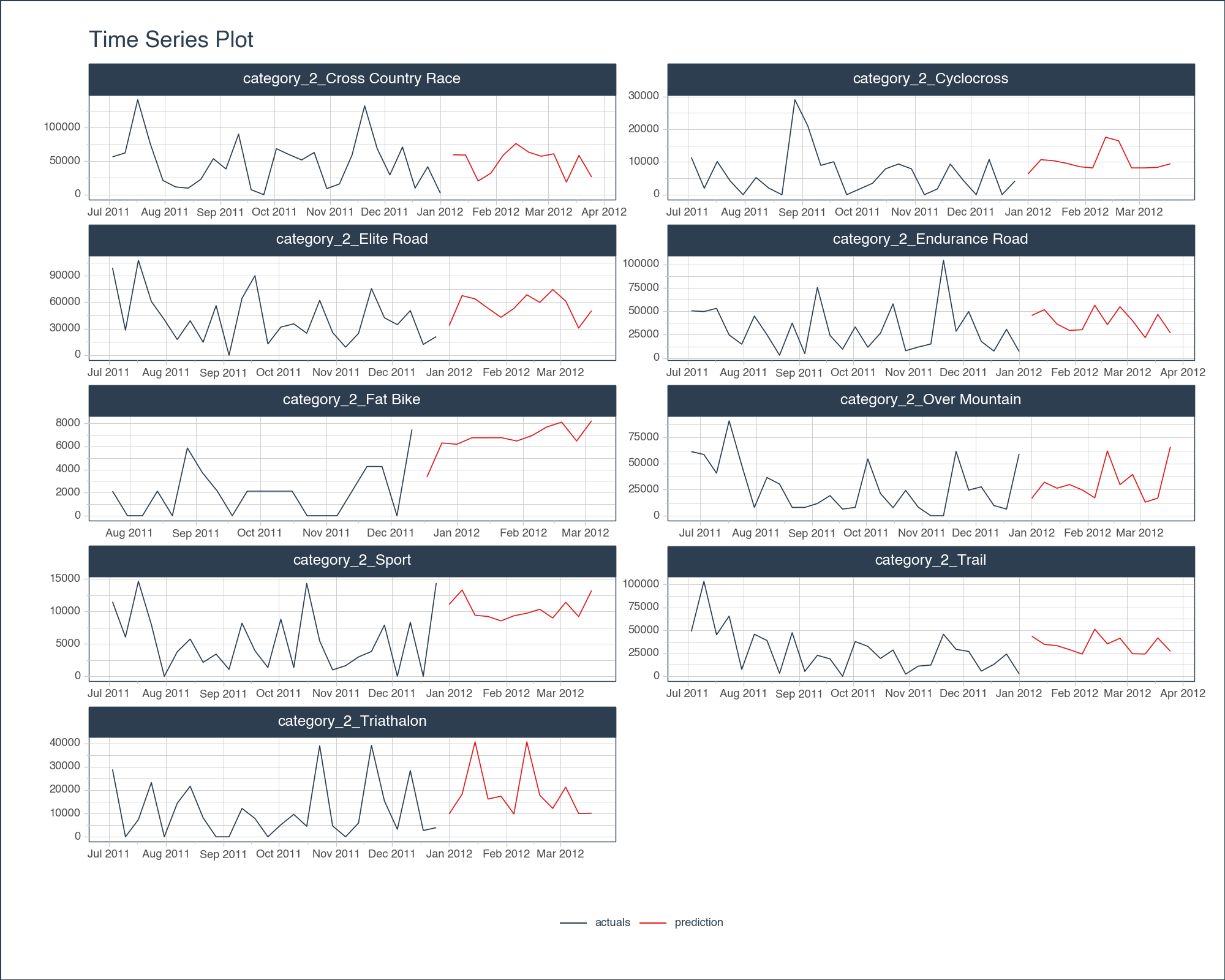
<Figure Size: (1000 x 800)>

Upon examining the graph, our models look alright given the length of time for training. Important points:

For effective time series forecasting, having multiple years of data is pivotal. This provides the model ample opportunities to recognize and adapt to seasonal variations.
Given our dataset spanned less than a year, the model lacked the depth of historical context to discern such patterns.
Although our feature engineering was kept basic to introduce various pytimetk capabilities, there’s room for enhancement.
For a more refined analysis, consider experimenting with different machine learning models and diving deeper into feature engineering.
Pytimetk’s tk.augment_fourier() might assist in discerning seasonal trends, but with the dataset’s limited historical scope, capturing intricate patterns could remain a challenge.

4 Conclusions

This was a great example of how pytimetk can help Data Analysts and Data Scientists examine sales patterns from Customer Relationship Management (CRM) Databases.

We examined ways to wrangle complex transactional data with tk.summarize_by_time
We discovered how to visualize customer and product data with tk.plot_timeseries
We used tk.pad_by_time and tk.future_frame to prepare data for modeling
And, we learned how to add many features with augment functions including tk.augment_timeseries_signature ant tk.agument_lags

All of these pytimetk skills and techniques were necessary to produce a good sales forecast with sklearn.

5 More Coming Soon…

We are in the early stages of development. But it’s obvious the potential for pytimetk now in Python. 🐍

Please ⭐ us on GitHub (it takes 2-seconds and means a lot).
To make requests, please see our Project Roadmap GH Issue #2. You can make requests there.
Want to contribute? See our contributing guide here.

1 Tutorial Setup

1.1 Load Packages.

1.2 Load & inspect dataset

2 Exploratory Analysis

2.1 Initial Inspection with tk.glimpse

2.2 Data Exploration with tk.summarize_by_time

Getting Weekly Totals

Get Weekly Totals by Group (Category 2)

Long vs Wide Format

2.3 Visualize your time series data with tk.plot_timeseries

3 Create a Product Forecast Model

3.1 Making irregular data regular with tk.pad_by_time

3.2 Making Future Dates Easier with tk.future_frame

3.3 Lag Values with tk.augment_lags

3.4 Date Features with tk.augment_timeseries_signature

One-Hot Encoding

Training and Future Feature Sets

3.5 Scikit Learn Model

Fitting a Random Forest Regressor

Prediction

Cleaning Up

Pre-Visualization Wrangling

Visualize the Forecast

4 Conclusions

5 More Coming Soon…

2.1 Initial Inspection with `tk.glimpse`

2.2 Data Exploration with `tk.summarize_by_time`

2.3 Visualize your time series data with `tk.plot_timeseries`

3.1 Making irregular data regular with `tk.pad_by_time`

3.2 Making Future Dates Easier with `tk.future_frame`

3.3 Lag Values with `tk.augment_lags`

3.4 Date Features with `tk.augment_timeseries_signature`