Autoregressive Forecasting with Recursive

Turn any tidymodel into an Autoregressive Forecasting Model

This short tutorial shows how you can use recursive() to:

• Make a Recursive Forecast Model for forecasting with short-term lags (i.e. Lag Size < Forecast Horizon).

• Perform Recursive Panel Forecasting, which is when you have a single autoregressive model that predicts forecasts for multiple time series.

Recursive Panel Forecast with XGBoost

Forecasting with Recursive Ensembles

We have a separate modeltime.ensemble package that includes support for recursive(). Making recursive ensembles is covered in the “Forecasting with Recursive Ensembles” article.

What is a Recursive Model?

A recursive model uses predictions to generate new values for independent features. These features are typically lags used in autoregressive models.

Why is Recursive needed for Autoregressive Models?

It’s important to understand that a recursive model is only needed when using lagged features with a Lag Size < Forecast Horizon. When the lag length is less than the forecast horizon, a problem exists were missing values (NA) are generated in the future data.

A solution that recursive() implements is to iteratively fill these missing values in with values generated from predictions. This technique can be used for:

1. Single time series predictions - Effectively turning any tidymodels model into an Autoregressive (AR) model

2. Panel time series predictions - In many situations we need to forecast more than one time series. We can batch-process these with 1 model by processing time series groups as panels. This technique can be extended to recursive forecasting for scalable models (1 model that predicts many time series).

Libraries

Load the following libraries.

library(modeltime)
library(tidymodels)
library(tidyverse)
library(timetk)

Make a Recursive Forecast Model

We’ll start with the simplest example, turning a Linear Regresion into an Autoregressive model.

Data Visualization

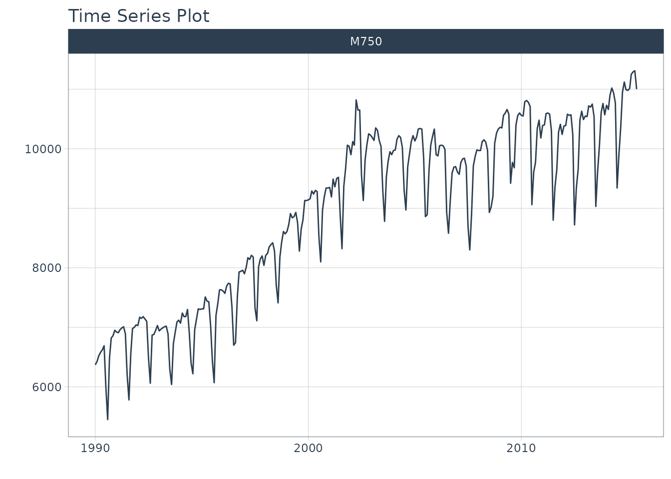
Let’s start with the m750 dataset.

m750
#> # A tibble: 306 × 3
#>    id    date       value
#>    <fct> <date>     <dbl>
#>  1 M750  1990-01-01  6370
#>  2 M750  1990-02-01  6430
#>  3 M750  1990-03-01  6520
#>  4 M750  1990-04-01  6580
#>  5 M750  1990-05-01  6620
#>  6 M750  1990-06-01  6690
#>  7 M750  1990-07-01  6000
#>  8 M750  1990-08-01  5450
#>  9 M750  1990-09-01  6480
#> 10 M750  1990-10-01  6820
#> # ℹ 296 more rows

We can visualize the data with plot_time_series().

m750 %>% 
  plot_time_series(
    .date_var    = date,
    .value       = value,
    .facet_var   = id,
    .smooth      = FALSE,
    .interactive = FALSE
  )

Data Preparation

Let’s establish a forecast horizon and extend the dataset to create a forecast region.

FORECAST_HORIZON <- 24

m750_extended <- m750 %>%
    group_by(id) %>%
    future_frame(
        .length_out = FORECAST_HORIZON,
        .bind_data  = TRUE
    ) %>%
    ungroup()

Transform Function

We’ll use short-term lags, lags with a size that are smaller than the forecast horizon. Here we create a custom function, lag_roll_transformer() that takes a dataset and adds lags 1 through 12 and a rolling mean using lag 12. Each of the features this function use lags less than our forecast horizon of 24 months, which means we need to use recursive().

lag_roll_transformer <- function(data){
    data %>%
        tk_augment_lags(value, .lags = 1:FORECAST_HORIZON) %>%
        tk_augment_slidify(
          contains("lag12"),
          .f = ~mean(.x, na.rm = TRUE),
          .period  = 12,
          .partial = TRUE
        ) 
}

Apply the Transform Function

When we apply the lag roll transformation to our extended data set, we can see the effect.

m750_rolling <- m750_extended %>%
    lag_roll_transformer() %>%
    select(-id)

m750_rolling
#> # A tibble: 330 × 27
#>    date       value value_lag1 value_lag2 value_lag3 value_lag4 value_lag5
#>    <date>     <dbl>      <dbl>      <dbl>      <dbl>      <dbl>      <dbl>
#>  1 1990-01-01  6370         NA         NA         NA         NA         NA
#>  2 1990-02-01  6430       6370         NA         NA         NA         NA
#>  3 1990-03-01  6520       6430       6370         NA         NA         NA
#>  4 1990-04-01  6580       6520       6430       6370         NA         NA
#>  5 1990-05-01  6620       6580       6520       6430       6370         NA
#>  6 1990-06-01  6690       6620       6580       6520       6430       6370
#>  7 1990-07-01  6000       6690       6620       6580       6520       6430
#>  8 1990-08-01  5450       6000       6690       6620       6580       6520
#>  9 1990-09-01  6480       5450       6000       6690       6620       6580
#> 10 1990-10-01  6820       6480       5450       6000       6690       6620
#> # ℹ 320 more rows
#> # ℹ 20 more variables: value_lag6 <dbl>, value_lag7 <dbl>, value_lag8 <dbl>,
#> #   value_lag9 <dbl>, value_lag10 <dbl>, value_lag11 <dbl>, value_lag12 <dbl>,
#> #   value_lag13 <dbl>, value_lag14 <dbl>, value_lag15 <dbl>, value_lag16 <dbl>,
#> #   value_lag17 <dbl>, value_lag18 <dbl>, value_lag19 <dbl>, value_lag20 <dbl>,
#> #   value_lag21 <dbl>, value_lag22 <dbl>, value_lag23 <dbl>, value_lag24 <dbl>,
#> #   value_lag12_roll_12 <dbl>

Split into Training and Future Data

The training data needs to be completely filled in. We remove any rows with NA.

train_data <- m750_rolling %>%
    drop_na()

train_data
#> # A tibble: 282 × 27
#>    date       value value_lag1 value_lag2 value_lag3 value_lag4 value_lag5
#>    <date>     <dbl>      <dbl>      <dbl>      <dbl>      <dbl>      <dbl>
#>  1 1992-01-01  7030       7040       7000       6980       6550       5780
#>  2 1992-02-01  7170       7030       7040       7000       6980       6550
#>  3 1992-03-01  7150       7170       7030       7040       7000       6980
#>  4 1992-04-01  7180       7150       7170       7030       7040       7000
#>  5 1992-05-01  7140       7180       7150       7170       7030       7040
#>  6 1992-06-01  7100       7140       7180       7150       7170       7030
#>  7 1992-07-01  6490       7100       7140       7180       7150       7170
#>  8 1992-08-01  6060       6490       7100       7140       7180       7150
#>  9 1992-09-01  6870       6060       6490       7100       7140       7180
#> 10 1992-10-01  6880       6870       6060       6490       7100       7140
#> # ℹ 272 more rows
#> # ℹ 20 more variables: value_lag6 <dbl>, value_lag7 <dbl>, value_lag8 <dbl>,
#> #   value_lag9 <dbl>, value_lag10 <dbl>, value_lag11 <dbl>, value_lag12 <dbl>,
#> #   value_lag13 <dbl>, value_lag14 <dbl>, value_lag15 <dbl>, value_lag16 <dbl>,
#> #   value_lag17 <dbl>, value_lag18 <dbl>, value_lag19 <dbl>, value_lag20 <dbl>,
#> #   value_lag21 <dbl>, value_lag22 <dbl>, value_lag23 <dbl>, value_lag24 <dbl>,
#> #   value_lag12_roll_12 <dbl>

The future data has missing values in the “value” column. We isolate these. Our autoregressive algorithm will predict these. Notice that the lags have missing data, this is OK - and why we are going to use recursive() to fill these missing values in with predictions.

future_data <- m750_rolling %>%
    filter(is.na(value))

future_data
#> # A tibble: 24 × 27
#>    date       value value_lag1 value_lag2 value_lag3 value_lag4 value_lag5
#>    <date>     <dbl>      <dbl>      <dbl>      <dbl>      <dbl>      <dbl>
#>  1 2015-07-01    NA      11000      11310      11290      11250      11010
#>  2 2015-08-01    NA         NA      11000      11310      11290      11250
#>  3 2015-09-01    NA         NA         NA      11000      11310      11290
#>  4 2015-10-01    NA         NA         NA         NA      11000      11310
#>  5 2015-11-01    NA         NA         NA         NA         NA      11000
#>  6 2015-12-01    NA         NA         NA         NA         NA         NA
#>  7 2016-01-01    NA         NA         NA         NA         NA         NA
#>  8 2016-02-01    NA         NA         NA         NA         NA         NA
#>  9 2016-03-01    NA         NA         NA         NA         NA         NA
#> 10 2016-04-01    NA         NA         NA         NA         NA         NA
#> # ℹ 14 more rows
#> # ℹ 20 more variables: value_lag6 <dbl>, value_lag7 <dbl>, value_lag8 <dbl>,
#> #   value_lag9 <dbl>, value_lag10 <dbl>, value_lag11 <dbl>, value_lag12 <dbl>,
#> #   value_lag13 <dbl>, value_lag14 <dbl>, value_lag15 <dbl>, value_lag16 <dbl>,
#> #   value_lag17 <dbl>, value_lag18 <dbl>, value_lag19 <dbl>, value_lag20 <dbl>,
#> #   value_lag21 <dbl>, value_lag22 <dbl>, value_lag23 <dbl>, value_lag24 <dbl>,
#> #   value_lag12_roll_12 <dbl>

Modeling

We’ll make 2 models for comparison purposes:

1. Straight-Line Forecast Model using Linear Regression with the Date feature
2. Autoregressive Forecast Model using Linear Regression with the Date feature, Lags 1-12, and Rolling Mean Lag 12

Model 1 (Baseline): Straight-Line Forecast Model

A straight-line forecast is just to illustrate the effect of no autoregressive features. Consider this a NAIVE modeling approach. The only feature that is used as a dependent variable is the “date” column.

model_fit_lm <- linear_reg() %>%
    set_engine("lm") %>%
    fit(value ~ date, data = train_data)

model_fit_lm
#> parsnip model object
#> 
#> 
#> Call:
#> stats::lm(formula = value ~ date, data = data)
#> 
#> Coefficients:
#> (Intercept)         date  
#>   3356.7208       0.4712

Model 2: Autoregressive Forecast Model

The autoregressive forecast model is simply a parsnip model with one additional step: using recursive(). The key components are:

• transform: A transformation function. We use the function previously made that generated Lags 1 to 12 and the Rolling Mean Lag 12 features.

• train_tail: The tail of the training data, which must be as large as the lags used in the transform function (i.e. lag 12).

  • Train tail can be larger than the lag size used. Notice that we use the Forecast Horizon, which is size 24.
  • For Panel Data, we need to include the tail for each group. We have provided a convenient panel_tail() function.

• id (Optional): This is used to identify groups for Recursive Panel Data.

# Autoregressive Forecast
model_fit_lm_recursive <- linear_reg() %>%
    set_engine("lm") %>%
    fit(value ~ ., data = train_data) %>%
    # One additional step - use recursive()
    recursive(
        transform  = lag_roll_transformer,
        train_tail = tail(train_data, FORECAST_HORIZON)
    )

model_fit_lm_recursive
#> Recursive [parsnip model]
#> 
#> parsnip model object
#> 
#> 
#> Call:
#> stats::lm(formula = value ~ ., data = data)
#> 
#> Coefficients:
#>         (Intercept)                 date           value_lag1  
#>           164.14732              0.00677              0.61244  
#>          value_lag2           value_lag3           value_lag4  
#>             0.18402             -0.07128              0.12089  
#>          value_lag5           value_lag6           value_lag7  
#>            -0.01750              0.07095              0.09785  
#>          value_lag8           value_lag9          value_lag10  
#>            -0.08053              0.04887              0.03030  
#>         value_lag11          value_lag12          value_lag13  
#>            -0.01755              0.73318             -0.52958  
#>         value_lag14          value_lag15          value_lag16  
#>            -0.21410              0.07734             -0.13879  
#>         value_lag17          value_lag18          value_lag19  
#>             0.04351             -0.08894             -0.08732  
#>         value_lag20          value_lag21          value_lag22  
#>             0.06641             -0.05737             -0.02331  
#>         value_lag23          value_lag24  value_lag12_roll_12  
#>             0.05754              0.15960                   NA

Modeltime Forecasting Workflow

Once we have our fitted model, we can follow the Modeltime Workflow (note we are skipping calibration and refitting, but this can be performed to get confidence intervals):

First, we add fitted models to a Model Table using modeltime_table(). (Note - If your model description says “LM”, install the development version of modeltime, which has improved model descriptions for recursive models).

model_tbl <- modeltime_table(
    model_fit_lm,
    model_fit_lm_recursive
) 

model_tbl
#> # Modeltime Table
#> # A tibble: 2 × 3
#>   .model_id .model   .model_desc 
#>       <int> <list>   <chr>       
#> 1         1 <fit[+]> LM          
#> 2         2 <fit[+]> RECURSIVE LM

Next, we perform Forecast Evaluation using modeltime_forecast() and plot_modeltime_forecast().

model_tbl %>% 
  
    # Forecast using future data
    modeltime_forecast(
        new_data    = future_data,
        actual_data = m750
    ) %>%
  
    # Visualize the forecast
    plot_modeltime_forecast(
        .interactive        = FALSE,
        .conf_interval_show = FALSE
    )

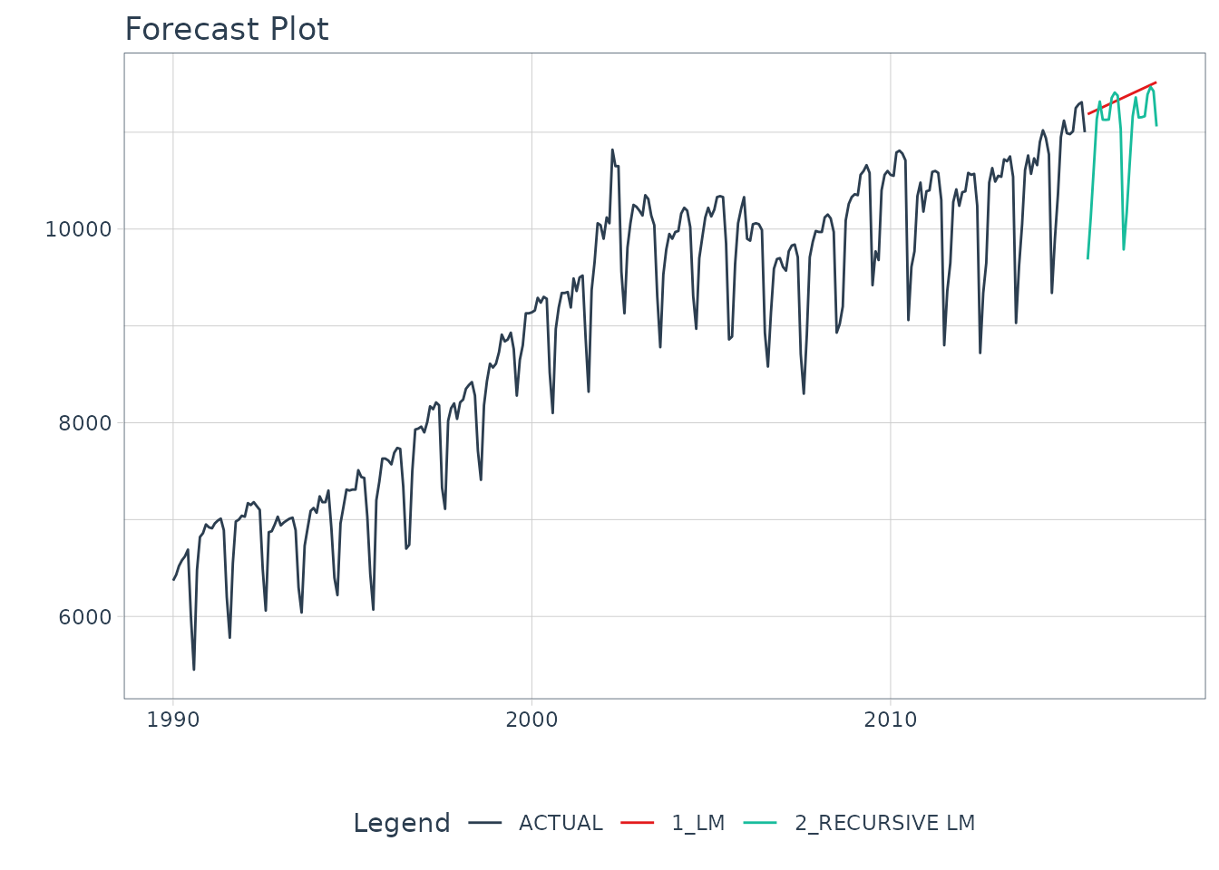
We can see the benefit of autoregressive features.

Recursive Forecasting with Panel Models

We can take this further by extending what we’ve learned here to panel data:

Panel Data:

• Grouped transformation functions: lag_roll_transformer_grouped()
• recursive(): Using id and the panel_tail() function

More sophisticated algorithms:

• Instead of using a simple Linear Regression
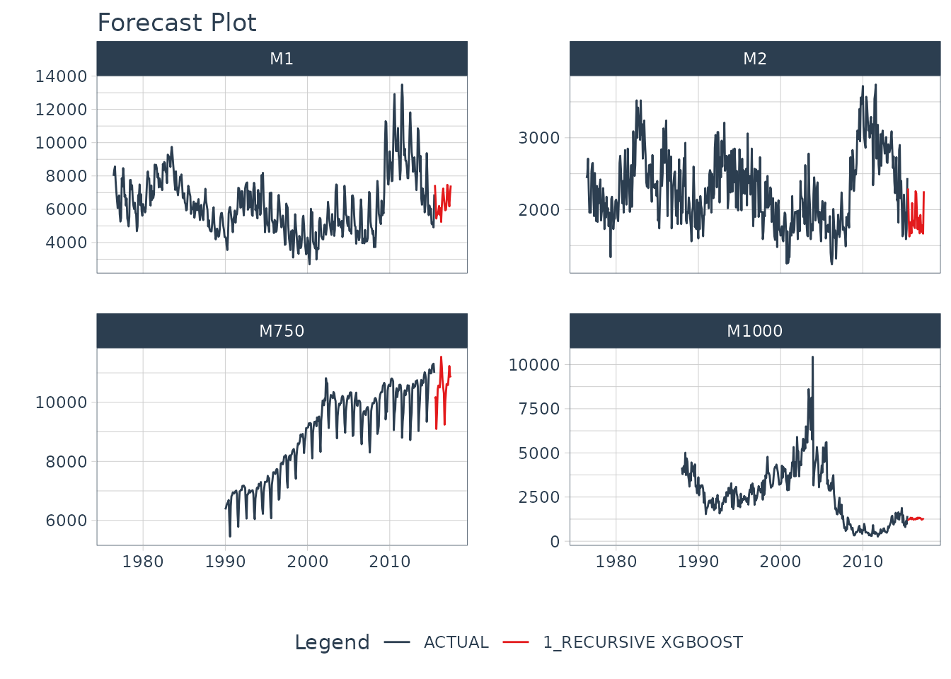
• We use xgboost to forecast multiple time series

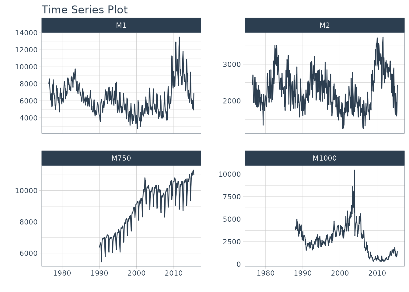
Data Visualization

Now we have 4 time series that we will forecast.

m4_monthly %>%  
  plot_time_series(
    .date_var    = date, 
    .value       = value, 
    .facet_var   = id, 
    .facet_ncol  = 2,
    .smooth      = FALSE, 
    .interactive = FALSE
)

Data Preparation

We use timetk::future_frame() to project each series forward by the forecast horizon. This sets up an extended data set with each series extended by 24 time stamps.

FORECAST_HORIZON <- 24

m4_extended <- m4_monthly %>%
    group_by(id) %>%
    future_frame(
        .length_out = FORECAST_HORIZON,
        .bind_data  = TRUE
    ) %>%
    ungroup()

Transform Function

The only difference is that we are applying any lags by group.

lag_roll_transformer_grouped <- function(data){
    data %>%
        group_by(id) %>%
        tk_augment_lags(value, .lags = 1:FORECAST_HORIZON) %>%
        tk_augment_slidify(
          .value   = contains("lag12"),
          .f       = ~mean(.x, na.rm = T),
          .period  = c(12),
          .partial = TRUE
        ) %>%
        ungroup()
}

Apply the Transform Function

We apply the groupwise lag transformation to the extended data set. This adds autoregressive features.

m4_lags <- m4_extended %>%
    lag_roll_transformer_grouped()

m4_lags
#> # A tibble: 1,670 × 28
#>    id    date       value value_lag1 value_lag2 value_lag3 value_lag4 value_lag5
#>    <fct> <date>     <dbl>      <dbl>      <dbl>      <dbl>      <dbl>      <dbl>
#>  1 M1    1976-06-01  8000         NA         NA         NA         NA         NA
#>  2 M1    1976-07-01  8350       8000         NA         NA         NA         NA
#>  3 M1    1976-08-01  8570       8350       8000         NA         NA         NA
#>  4 M1    1976-09-01  7700       8570       8350       8000         NA         NA
#>  5 M1    1976-10-01  7080       7700       8570       8350       8000         NA
#>  6 M1    1976-11-01  6520       7080       7700       8570       8350       8000
#>  7 M1    1976-12-01  6070       6520       7080       7700       8570       8350
#>  8 M1    1977-01-01  6650       6070       6520       7080       7700       8570
#>  9 M1    1977-02-01  6830       6650       6070       6520       7080       7700
#> 10 M1    1977-03-01  5710       6830       6650       6070       6520       7080
#> # ℹ 1,660 more rows
#> # ℹ 20 more variables: value_lag6 <dbl>, value_lag7 <dbl>, value_lag8 <dbl>,
#> #   value_lag9 <dbl>, value_lag10 <dbl>, value_lag11 <dbl>, value_lag12 <dbl>,
#> #   value_lag13 <dbl>, value_lag14 <dbl>, value_lag15 <dbl>, value_lag16 <dbl>,
#> #   value_lag17 <dbl>, value_lag18 <dbl>, value_lag19 <dbl>, value_lag20 <dbl>,
#> #   value_lag21 <dbl>, value_lag22 <dbl>, value_lag23 <dbl>, value_lag24 <dbl>,
#> #   value_lag12_roll_12 <dbl>

Split into Training and Future Data

Just like the single case, we split into future and training data.

train_data <- m4_lags %>%
    drop_na()

future_data <- m4_lags %>%
    filter(is.na(value))

Modeling

We’ll use a more sophisticated algorithm xgboost to develop an autoregressive model.

# Modeling Autoregressive Panel Data
set.seed(123)
model_fit_xgb_recursive <- boost_tree(
        mode = "regression",
        learn_rate = 0.35
    ) %>%
    set_engine("xgboost") %>%
    fit(
        value ~ . 
        + month(date, label = TRUE) 
        + as.numeric(date) 
        - date, 
        data = train_data
    ) %>%
    recursive(
        id         = "id", # We add an id = "id" to specify the groups
        transform  = lag_roll_transformer_grouped,
        # We use panel_tail() to grab tail by groups
        train_tail = panel_tail(train_data, id, FORECAST_HORIZON)
    )

model_fit_xgb_recursive
#> Recursive [parsnip model]
#> 
#> parsnip model object
#> 
#> ##### xgb.Booster
#> raw: 52.7 Kb 
#> call:
#>   xgboost::xgb.train(params = list(eta = 0.35, max_depth = 6, gamma = 0, 
#>     colsample_bytree = 1, colsample_bynode = 1, min_child_weight = 1, 
#>     subsample = 1), data = x$data, nrounds = 15, watchlist = x$watchlist, 
#>     verbose = 0, nthread = 1, objective = "reg:squarederror")
#> params (as set within xgb.train):
#>   eta = "0.35", max_depth = "6", gamma = "0", colsample_bytree = "1", colsample_bynode = "1", min_child_weight = "1", subsample = "1", nthread = "1", objective = "reg:squarederror", validate_parameters = "TRUE"
#> xgb.attributes:
#>   niter
#> callbacks:
#>   cb.evaluation.log()
#> # of features: 41 
#> niter: 15
#> nfeatures : 41 
#> evaluation_log:
#>     iter training_rmse
#>        1     3767.4588
#>        2     2494.2021
#> ---                   
#>       14      210.7798
#>       15      200.4422

Modeltime Forecasting Workflow

First, create a Modeltime Table. Note - If your model description says “XGBOOST”, install the development version of modeltime, which has improved model descriptions for recursive models).

model_tbl <- modeltime_table(
    model_fit_xgb_recursive
)

model_tbl
#> # Modeltime Table
#> # A tibble: 1 × 3
#>   .model_id .model   .model_desc      
#>       <int> <list>   <chr>            
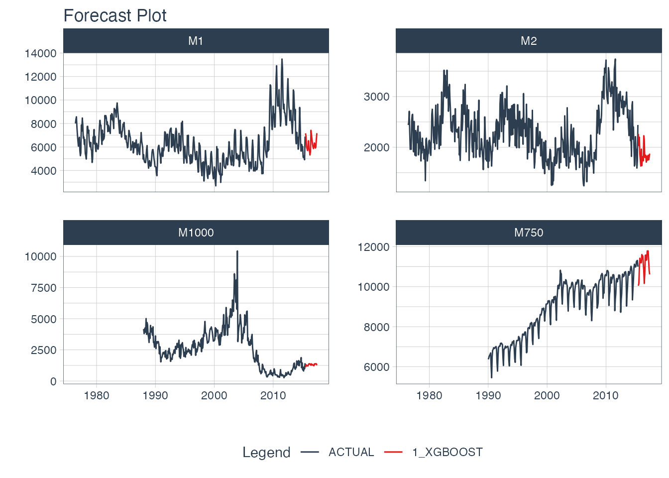
#> 1         1 <fit[+]> RECURSIVE XGBOOST

Next, we can forecast the results.

model_tbl %>%
    modeltime_forecast(
        new_data    = future_data,
        actual_data = m4_monthly,
        keep_data   = TRUE
    ) %>%
    group_by(id) %>%
    plot_modeltime_forecast(
        .interactive        = FALSE,
        .conf_interval_show = FALSE,
        .facet_ncol         = 2
    )

Summary

We just showcased Recursive Forecasting. But this is a simple problem. And, there’s a lot more to learning time series.

• Many more algorithms
• Ensembling
• Machine Learning
• Deep Learning
• Scalable Modeling: 10,000+ time series

Your probably thinking how am I ever going to learn time series forecasting. Here’s the solution that will save you years of struggling.

Take the High-Performance Forecasting Course

Become the forecasting expert for your organization

High-Performance Time Series Course

Time Series is Changing

Time series is changing. Businesses now need 10,000+ time series forecasts every day. This is what I call a High-Performance Time Series Forecasting System (HPTSF) - Accurate, Robust, and Scalable Forecasting.

High-Performance Forecasting Systems will save companies by improving accuracy and scalability. Imagine what will happen to your career if you can provide your organization a “High-Performance Time Series Forecasting System” (HPTSF System).

How to Learn High-Performance Time Series Forecasting

I teach how to build a HPTFS System in my High-Performance Time Series Forecasting Course. You will learn:

• Time Series Machine Learning (cutting-edge) with Modeltime - 30+ Models (Prophet, ARIMA, XGBoost, Random Forest, & many more)
• Deep Learning with GluonTS (Competition Winners)
• Time Series Preprocessing, Noise Reduction, & Anomaly Detection
• Feature engineering using lagged variables & external regressors
• Hyperparameter Tuning
• Time series cross-validation
• Ensembling Multiple Machine Learning & Univariate Modeling Techniques (Competition Winner)
• Scalable Forecasting - Forecast 1000+ time series in parallel
• and more.

Become the Time Series Expert for your organization.

Take the High-Performance Time Series Forecasting Course