Conformal Forecast Prediction Intervals in Modeltime • modeltime

Modeltime integrates Conformal Prediction Intervals as part of its time series forecasting workflow. This tutorial showcases 2 methods for Conformal Prediction Intervals:

Conformal Default Method: Uses qnorm() to compute quantiles from out-of-sample (test set) residuals.
Conformal Split Method Uses the split method split conformal inference method described by Lei et al (2018)

Time Series Conformal Forecasting Prediction Interval Tutorial

Load libraries to complete this short tutorial.

library(tidyverse)

library(tidymodels)
library(modeltime)
library(timetk)

# This toggles plots from plotly (interactive) to ggplot (static)
interactive <- FALSE

Step 1 - Collect data and split into training, test, and future data sets.

We’ll start with the Walmart Sales data set from timetk.

# Data

walmart_sales_tbl <- timetk::walmart_sales_weekly %>%
    select(id, Date, Weekly_Sales) %>%
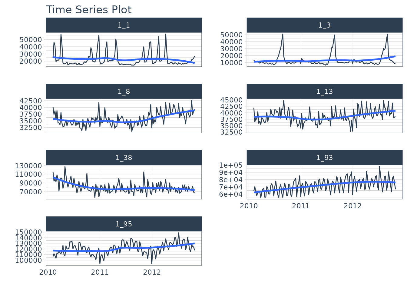
    mutate(id = forcats::as_factor(id))

We can visualize the data set.

walmart_sales_tbl %>%
    group_by(id) %>%
    plot_time_series(
        Date, Weekly_Sales,
        .facet_ncol  = 2,
        .interactive = interactive,
    )

Let’s split the data into training and test sets using time_series_split()

# Split Data 80/20
splits <- time_series_split(
    walmart_sales_tbl,
    assess     = "1 year",
    cumulative = TRUE
)

splits
#> <Analysis/Assess/Total>
#> <637/364/1001>

Finally, let’s make a future dataset that will be used to forecast the next 1 year.

new_data_tbl <- walmart_sales_tbl %>%
    group_by(id) %>%
    future_frame(.length_out = "1 year") %>%
    ungroup()

Step 2 - Create & Fit Forecasting Models

We’ll set up an XGBoost forecasting model for this tutorial.

Recipe

First, let’s create a recipe. This step creates a number of time series features and one-hot encodes any categorical features.

recipe_ml <- recipe(Weekly_Sales ~ ., training(splits)) %>%
    step_timeseries_signature(Date) %>%
    step_rm(Date) %>%
    step_dummy(all_nominal_predictors(), one_hot = TRUE)

recipe_ml

Model & Workflow

Next, let’s create the model and fit the recipe and model on the training dataset.

model_xgb <- boost_tree("regression") %>%
    set_engine("xgboost")

wflw_fit_xgb <- workflow() %>%
    add_model(model_xgb) %>%
    add_recipe(recipe_ml) %>%
    fit(training(splits))

wflw_fit_xgb
#> ══ Workflow [trained] ══════════════════════════════════════════════════════════
#> Preprocessor: Recipe
#> Model: boost_tree()
#> 
#> ── Preprocessor ────────────────────────────────────────────────────────────────
#> 3 Recipe Steps
#> 
#> • step_timeseries_signature()
#> • step_rm()
#> • step_dummy()
#> 
#> ── Model ───────────────────────────────────────────────────────────────────────
#> ##### xgb.Booster
#> raw: 44.1 Kb 
#> call:
#>   xgboost::xgb.train(params = list(eta = 0.3, max_depth = 6, gamma = 0, 
#>     colsample_bytree = 1, colsample_bynode = 1, min_child_weight = 1, 
#>     subsample = 1), data = x$data, nrounds = 15, watchlist = x$watchlist, 
#>     verbose = 0, nthread = 1, objective = "reg:squarederror")
#> params (as set within xgb.train):
#>   eta = "0.3", max_depth = "6", gamma = "0", colsample_bytree = "1", colsample_bynode = "1", min_child_weight = "1", subsample = "1", nthread = "1", objective = "reg:squarederror", validate_parameters = "TRUE"
#> xgb.attributes:
#>   niter
#> callbacks:
#>   cb.evaluation.log()
#> # of features: 3375 
#> niter: 15
#> nfeatures : 3375 
#> evaluation_log:
#>     iter training_rmse
#>        1     45890.002
#>        2     32737.320
#> ---                   
#>       14      3093.845
#>       15      2945.648

Step 3 - Add fitted models to a Model Table.

The next step is to add model(s) to a modeltime table. This step stores the model in a data frame for organizational purposes.

models_tbl <- modeltime_table(
     wflw_fit_xgb
)

models_tbl
#> # Modeltime Table
#> # A tibble: 1 × 3
#>   .model_id .model     .model_desc
#>       <int> <list>     <chr>      
#> 1         1 <workflow> XGBOOST

Step 4 - Calibrate the model to a testing set.

Next, we calibrate the model using the testing set. Note- I’m using the id = "id" which allows us to track confidence for each time series group in our dataset. The column “id” is used as the grouping column.

calibration_tbl <- models_tbl %>%
    modeltime_calibrate(
        new_data = testing(splits), 
        id       = "id"
    )

calibration_tbl
#> # Modeltime Table
#> # A tibble: 1 × 5
#>   .model_id .model     .model_desc .type .calibration_data 
#>       <int> <list>     <chr>       <chr> <list>            
#> 1         1 <workflow> XGBOOST     Test  <tibble [364 × 5]>

Conformal Prediction

With the calibration table in hand, we can now implement the conformal prediction interval. Currently, there are 2 methods implemented in modeltime_forecast:

conformal_default: Uses qnorm() to compute quantiles from out-of-sample (test set) residuals.
conformal_split: Uses the split method split conformal inference method described by Lei et al (2018)

Conformal Default Method

The default method has been implemented in modeltime from the start of the modeltime package.

This method uses qnorm() to produce a 95% confidence interval by default. It estimates a normal (Gaussian distribution) based on the out-of-sample errors (residuals).
The confidence interval is mean-adjusted, meaning that if the mean of the residuals is non-zero, the confidence interval is adjusted to widen the interval to capture the difference in means.

Here we implement a 95% confidence interval meaning 95% of the test data will fall within the boundaries. The tail() function is used to show the .conf_lo and .conf_hi probabilistic prediction intervals.

forecast_tbl <- calibration_tbl %>%
    modeltime_forecast(
        new_data      = testing(splits),
        actual_data   = walmart_sales_tbl,
        conf_interval = 0.95,
        conf_method   = "conformal_default", # Default Conformal Method
        conf_by_id    = TRUE, # TRUE = local CI by ID, FALSE = global CI
        keep_data     = TRUE
    )

# Last 7 data points for (1 for each time series)
forecast_tbl %>% tail(7)
#> # Forecast Results
#>   # A tibble: 7 × 10
#>   .model_id .model_desc .key       .index      .value .conf_lo .conf_hi id   
#>       <int> <chr>       <fct>      <date>       <dbl>    <dbl>    <dbl> <fct>
#> 1         1 XGBOOST     prediction 2012-10-26  24996.   10825.   39167. 1_1  
#> 2         1 XGBOOST     prediction 2012-10-26  10884.    4842.   16927. 1_3  
#> 3         1 XGBOOST     prediction 2012-10-26  33634.   25973.   41296. 1_8  
#> 4         1 XGBOOST     prediction 2012-10-26  37287.   31689.   42884. 1_13 
#> 5         1 XGBOOST     prediction 2012-10-26  69167.   49454.   88880. 1_38 
#> 6         1 XGBOOST     prediction 2012-10-26  63422.   47315.   79529. 1_93 
#> 7         1 XGBOOST     prediction 2012-10-26 111583.   95210.  127956. 1_95 
#> # ℹ 2 more variables: Date <date>, Weekly_Sales <dbl>

We can visualize the probability intervals for the Conformal Default method.

forecast_tbl %>%
    group_by(id) %>%
    plot_modeltime_forecast(
        .facet_ncol  = 2, 
        .interactive = interactive,
        .title       = "Conformal Default"
    )

Conformal Split Method

When conf_method = "conformal_split, this method uses the split conformal inference method described by Lei et al (2018). This is also implemented in the probably R package’s int_conformal_split() function.

forecast_tbl <- calibration_tbl %>%
    modeltime_forecast(
        new_data      = testing(splits),
        actual_data   = walmart_sales_tbl,
        conf_interval = 0.95,
        conf_method   = "conformal_split", # Split Conformal Method
        conf_by_id    = TRUE, # TRUE = local CI by ID, FALSE = global CI
        keep_data     = TRUE
    )

# Last 7 data points for (1 for each time series)
forecast_tbl %>% tail(7)
#> # Forecast Results
#>   # A tibble: 7 × 10
#>   .model_id .model_desc .key       .index      .value .conf_lo .conf_hi id   
#>       <int> <chr>       <fct>      <date>       <dbl>    <dbl>    <dbl> <fct>
#> 1         1 XGBOOST     prediction 2012-10-26  24996.    8291.   41701. 1_1  
#> 2         1 XGBOOST     prediction 2012-10-26  10884.    3173.   18596. 1_3  
#> 3         1 XGBOOST     prediction 2012-10-26  33634.   26540.   40729. 1_8  
#> 4         1 XGBOOST     prediction 2012-10-26  37287.   32028.   42545. 1_13 
#> 5         1 XGBOOST     prediction 2012-10-26  69167.   51069.   87265. 1_38 
#> 6         1 XGBOOST     prediction 2012-10-26  63422.   46734.   80110. 1_93 
#> 7         1 XGBOOST     prediction 2012-10-26 111583.   94681.  128486. 1_95 
#> # ℹ 2 more variables: Date <date>, Weekly_Sales <dbl>

We can visualize the probability intervals for the Conformal Split method.

forecast_tbl %>%
    group_by(id) %>%
    plot_modeltime_forecast(
        .facet_ncol  = 2, 
        .interactive = interactive,
        .title       = "Conformal Split"
    )

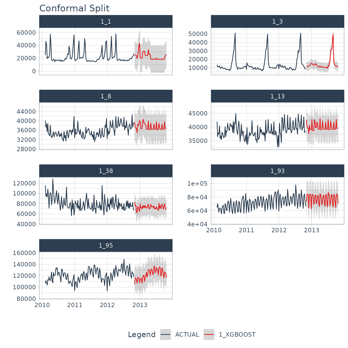
Refit and Future Forecast

Many Conformal Prediction tutorials fail to show how to make the future forecast for data that has not happened yet. I aim to fix this. Using the following code, we can quickly refit the model and make the future forecast applying the conformal probabilities to the future forecast estimates.

refit_tbl <- calibration_tbl %>%
    modeltime_refit(walmart_sales_tbl)

forecast_future_tbl <- refit_tbl %>%
    modeltime_forecast(
        new_data      = new_data_tbl,
        actual_data   = walmart_sales_tbl,
        conf_interval = 0.95,
        conf_method   = "conformal_split", # Split Conformal Method
        conf_by_id    = TRUE, # TRUE = local CI by ID, FALSE = global CI
        keep_data     = TRUE
    )

With the future forecast, we can visualize both the point estimates and the 95% conformal probability region.

forecast_future_tbl %>%
    group_by(id) %>%
    plot_modeltime_forecast(
        .facet_ncol  = 2, 
        .interactive = interactive,
        .title       = "Conformal Split"
    )

Summary

You have just seen how to do a simple Conformal Prediction estimate for a global time series model. But this is a simple problem. And, there’s a lot more to learning time series.

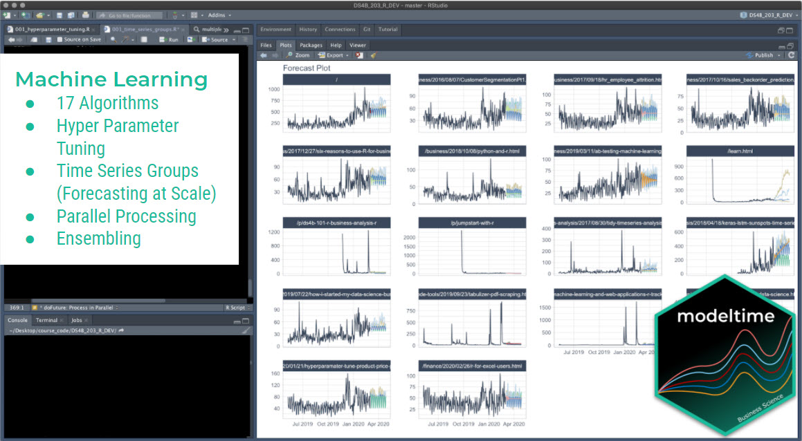
Many more algorithms
Ensembling
Machine Learning
Deep Learning
Iterative Forecasting
Scalable Modeling: 10,000+ time series

Your probably thinking how am I ever going to learn time series forecasting. Here’s the solution that will save you years of struggling.

Take the High-Performance Forecasting Course

Become the forecasting expert for your organization

High-Performance Time Series Course

Time Series is Changing

Time series is changing. Businesses now need 10,000+ time series forecasts every day. This is what I call a High-Performance Time Series Forecasting System (HPTSF) - Accurate, Robust, and Scalable Forecasting.

High-Performance Forecasting Systems will save companies by improving accuracy and scalability. Imagine what will happen to your career if you can provide your organization a “High-Performance Time Series Forecasting System” (HPTSF System).

How to Learn High-Performance Time Series Forecasting

I teach how to build a HPTFS System in my High-Performance Time Series Forecasting Course. You will learn:

Time Series Machine Learning (cutting-edge) with Modeltime - 30+ Models (Prophet, ARIMA, XGBoost, Random Forest, & many more)
Deep Learning with GluonTS (Competition Winners)
Time Series Preprocessing, Noise Reduction, & Anomaly Detection
Feature engineering using lagged variables & external regressors
Hyperparameter Tuning
Time series cross-validation
Ensembling Multiple Machine Learning & Univariate Modeling Techniques (Competition Winner)
Scalable Forecasting - Forecast 1000+ time series in parallel
and more.

Become the Time Series Expert for your organization.

Take the High-Performance Time Series Forecasting Course