Extending Modeltime (Developer Tools)

Introduction

The modeltime package was with extensibility in mind. It’s impossible to incorporate the entire R time series ecosystem into a single package. More than likely your going to need something that hasn’t been included yet. And, if you’re a developer, I challenge you to extend modeltime to suit your needs. I’ve spent a lot of time thinking about:

• A systematic workflow that can be used for time series analysis
• A way to integrate time series into a best-in-class modeling framework (i.e. tidymodels)

And, I want you to leverage what has been built so you don’t have to recreate the wheel.

Before we get started, where are we coming from?

Beyond being an amazing ecosystem for Machine Learning analysis in R, tidymodels is a developer-friendly infrastructure that enables parsnip-adjacent packages like modeltime. The ecosystem provides basic building blocks for extending machine learning models, tuning parameters, performance metrics, and preprocessing (feature engineering) tools. Before you start building, I highly recommend reviewing these resources:

• Parsnip Models (Algorithms): How to build a parsnip model
• Dials Parameters (Tuning): How to create a tuning parameter function
• Yardstick Metrics (Performance): Custom performance metrics
• Recipes Step Functions (preprocessing): Create your own recipe step function

The most important is the first resource - “How to build a parsnip model”.

Where we are going!

What we’re going to do momentarily is modify the “How to build a parsnip model” article. Your learning “How to build a modeltime model”. There are a few key nuances:

1. Managing Date and Date-time Features
2. Processing Regressors and Dates separately

Example
Integrating Multiple Seasonal Decomposition

The forecast package includes the stlm() function for creating models using time series decomposition. It’s a great approach based on the concept that you can decompose complex seasonality into multiple components:

• Trend
• One or Multiple Seasonalities
• Remainder

We can then forecast the components using models like: auto.arima() and ets().

Note - I’ve added a seasonal_reg() function that includes the functionality we are about to create. Check that function out to see more about seasonal decomposition methods.

Libraries

To use the code in this tutorial, you’ll need to have the following packages installed.

library(parsnip)
library(forecast)
library(rsample)
library(modeltime)
library(tidyverse)
library(timetk)
library(rlang)

Data

We’ll use taylor_30_min data from the timetk package, which is electricity demand data at a 30-minute interval.

taylor_30_min %>%
  plot_time_series(date, value, .interactive = FALSE)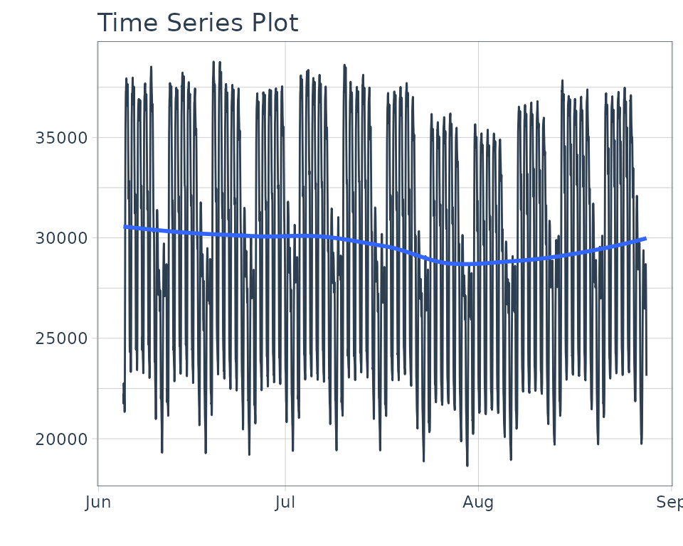

STLM Model - A quick overview

We need to use 2 functions to create the model:

• msts() - Tracks the multiple-seasonality as an object
• stlm() - Creates a model from the msts object.

Note that we use seasonal periods (24*2 = 48) for daily seasonality because this series has been aggregated at a 30-minute interval. The second seasonality is at 7-days, so we just use 24*2*7.

stlm_model <- taylor_30_min %>%
  pull(value) %>%
  msts(seasonal.periods = c(24*2, 24*2*7)) %>%
  stlm()

stlm_model$stl %>% autoplot()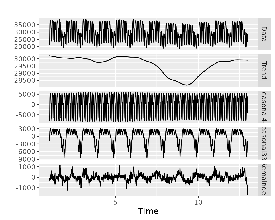

The forecast() function is used to generate predictions, much like the predict() function.

stlm_model %>%
  forecast(h = 24*2*7) %>%
  autoplot()

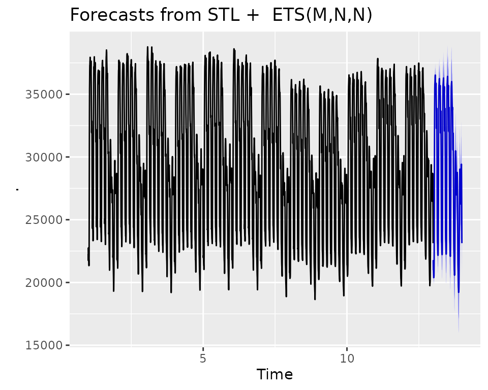
Looks like it’s doing a pretty decent job of forecasting the Taylor 30-Min Data.

How to build a modeltime model

The first step we need to do is to think about the function. We can create:

• msts(): Creates a multiple time series object. Key arguments: seasonal.periods.
• stlm(): Creates the Multiple STL Model. Key arguments:
  • method: Either ets or arima (actually uses auto.arima)
  • We’ll handle this by creating a specific engine called “stlm_ets” for the ets version.

We could add others, but let’s keep it simple for now.

The General Process

We follow a very similar process to “How to build a parsnip model” with a few additional aspects:

1. We create a “Modeltime Bridge” function to bridge between parsnip api functions and forecast time series.
2. We handle feature preprocessing internally to the model bridge to avoid the issue of losing dates and date-time information.

Step 1: Register the Model, Modes, and Arguments

Let’s add a new model called decomposition_reg() for Regression by Decomposition. Because Time Series analysis is generally regression, we’ll just register the regression mode.

set_new_model("decomposition_reg")
set_model_mode(model = "decomposition_reg", mode = "regression")
set_model_engine(model = "decomposition_reg", mode = "regression", eng = "stlm_ets")

# Here we set the dependency to forecast, though we can also use
# your package if you import the lower level package
set_dependency(model = "decomposition_reg", eng = "stlm_ets", pkg = "forecast")

We can use show_model_info() to see what’s been added to the registered model.

show_model_info("decomposition_reg")
#> Information for `decomposition_reg`
#>  modes: unknown, regression 
#> 
#>  engines: 
#>    regression: stlm_etsNA
#> 
#> ¹The model can use case weights.
#> 
#>  no registered arguments.
#> 
#>  no registered fit modules.
#> 
#>  no registered prediction modules.

We need to add model arguments as well. We’ll use set_model_args() to add the appropriate model arguments.

# 1st Frequency (period_seasonal_1 is a non-jargony term)
set_model_arg(
  model        = "decomposition_reg", 
  eng          = "stlm_ets", 
  parsnip      = "period_seasonal_1", 
  original     = "period_seasonal_1", 
  func         = list(pkg = "foo", fun = "bar"),
  has_submodel = FALSE
)

# 2nd Frequency (period_seasonal_2 is a non-jargony term)
set_model_arg(
  model        = "decomposition_reg", 
  eng          = "stlm_ets", 
  parsnip      = "period_seasonal_2", 
  original     = "period_seasonal_2", 
  func         = list(pkg = "foo", fun = "bar"),
  has_submodel = FALSE
)

Important note: We are going to map these “modeltime” arguments to a lower-level bridge function, so we don’t need original = seasonal.periods. In fact, we can’t do this because you need to have a one-to-one relationship between your parsnip/modeltime model arguments and the lower-level modeling function.

Step 2: Create the model function

We’ll create a decomposition_reg() function that will be our core parsnip function.

decomposition_reg <- function(mode = "regression", 
                              period_seasonal_1 = NULL, 
                              period_seasonal_2 = NULL) {

    args <- list(
        period_seasonal_1 = rlang::enquo(period_seasonal_1),
        period_seasonal_2 = rlang::enquo(period_seasonal_2)
    )

    parsnip::new_model_spec(
        "decomposition_reg",
        args     = args,
        eng_args = NULL,
        mode     = mode,
        method   = NULL,
        engine   = NULL
    )

}

Step 3: Add a Fit Bridge & Module

For Time Series models, we need to do extra work to get them to fit the parsnip mold. The easiest way is to create a “Bridge” function that helps process the data and connect the arguments with the underlying time series package.

Step 3A: Create the Fit Bridge

Time Series Developer Tools come included with modeltime:

• Bridge Constructor: new_modeltime_bridge(), A constructor for creating modeltime bridges that provide the connection between time series models and the parsnip infrastructure.
• Xreg Preprocessing Tools: create_xreg_recipe(), juice_xreg_recipe(), and bake_xreg_recipe()
• Date and Date-Time Parsing Tools: parse_index_from_data(), parse_period_from_index()

Here’s a sample bridge function. It:

1. Handles the data inputs, x (data.frame of predictors) and y (vector, target)
2. Handles the timestamp data (index) - This column is parsed from x
3. Handles the Predictors - formatting as necessary. The ets() model is univariate, so no predictors are necessary to be transformed.
   
4. Handles Fitting the model
5. Creates a new model bridge using the constructor, new_modeltime_bridge()

bridge_stlm_ets_fit_impl <- function(x, y, period_seasonal_1 = NULL, period_seasonal_2 = NULL, ...) {
  
  outcome    <- y # Comes in as a vector
  predictors <- x # Comes in as a data.frame (dates and possible xregs)
  
  # 1. Create outcome msts object by mapping `period_seasonal` args to msts()
  if (is.null(period_seasonal_1) || period_seasonal_1 <= 1) {
    stop("'period_seasonal_1' must be greater than 1 to assess seasonality")
  } else if (is.null(period_seasonal_2) || period_seasonal_2 <= 1) {
    seasonal.periods <- period_seasonal_1
  } else {
    seasonal.periods <- c(period_seasonal_1, period_seasonal_2)
  }
  outcome_msts <- forecast::msts(outcome, seasonal.periods = seasonal.periods)
  
  # 2. Predictors - Handle Dates 
  index_tbl <- parse_index_from_data(predictors)
  idx_col   <- names(index_tbl)
  idx       <- timetk::tk_index(index_tbl)
  
  # 3. Predictors - Handle Xregs
  # NOT REQUIRED - ETS is univariate
  # REQUIRED FOR ARIMA - ARIMA can accept XRegs
  # xreg_recipe <- create_xreg_recipe(predictor, prepare = TRUE)
  # xreg_matrix <- juice_xreg_recipe(xreg_recipe, format = "matrix")
  
  # 4. Fitting
  model_1 <- forecast::stlm(y = outcome_msts, method = "ets", ...)
  
  # 5. New Modeltime Bridge
  new_modeltime_bridge(
    class  = "bridge_stlm_ets_fit_impl",
    models = list(model_1 = model_1),
    data   = tibble(
      idx_col   := idx,
      .actual    = y,
      .fitted    = model_1$fitted,
      .residuals = model_1$residuals
    ),
    extras = list(NULL), # Can add xreg preprocessors here
    desc   = str_c("STLM Model: ", model_1$model$method)
  )
  
}

We’ll make a quick print method so we don’t get crazy output.

print.bridge_stlm_ets_fit_impl <- function(x, ...) {
  
  model <- x$models$model_1$model
  
  cat(x$desc)
  cat("\n")
  print(model$call)
  cat("\n")
  print(
    tibble(
      aic    = model$aic,
      bic    = model$bic,
      aicc   = model$aicc,
      loglik = model$loglik,
      mse    = model$mse  
    )
  )
  invisible(x)
}

Let’s make sure our bridge works.

stlm_test <- bridge_stlm_ets_fit_impl(
  x = taylor_30_min[,"date"],
  y = taylor_30_min %>% pull(value),
  period_seasonal_1 = 24*2,
  period_seasonal_2 = 24*2*7
)

stlm_test
#> STLM Model: ETS(M,N,N)
#> ets(y = x, model = etsmodel, allow.multiplicative.trend = allow.multiplicative.trend)
#> 
#> # A tibble: 1 × 5
#>      aic    bic   aicc  loglik   mse
#>    <dbl>  <dbl>  <dbl>   <dbl> <dbl>
#> 1 70395. 70414. 70395. -35194. 9501.

The bridge looks good.

Step 3B: Create a Fit Module

Next, let’s hook up our parsnip fit module to the newly created bridge fit function.

set_fit(
  model  = "decomposition_reg",
  eng    = "stlm_ets",
  mode   = "regression",
  value  = list(
    interface = "data.frame",
    protect   = c("x", "y"),
    func      = c(fun = "bridge_stlm_ets_fit_impl"),
    defaults  = list()
  )
)

show_model_info("decomposition_reg")
#> Information for `decomposition_reg`
#>  modes: unknown, regression 
#> 
#>  engines: 
#>    regression: stlm_ets
#> 
#> ¹The model can use case weights.
#> 
#>  arguments: 
#>    stlm_ets: 
#>       period_seasonal_1 --> period_seasonal_1
#>       period_seasonal_2 --> period_seasonal_2
#> 
#>  fit modules:
#>      engine       mode
#>    stlm_ets regression
#> 
#>  no registered prediction modules.

Step 4: Add a Prediction Bridge & Module

Next, we have an additional step to bridge the prediction. We create a predict method that handles the new_data, treating the number of rows as the forecasting horizon.

Step 4A: Create a Prediction Bridge

predict.bridge_stlm_ets_fit_impl <- function(object, new_data, ...) {

    # PREPARE INPUTS
    model       <- object$models$model_1
    h_horizon   <- nrow(new_data)

    # XREG
    # NOT REQUIRED FOR ETS. 
    # xreg_recipe <- object$extras$xreg_recipe 
    # xreg_matrix <- bake_xreg_recipe(xreg_recipe, new_data, format = "matrix")

    # PREDICTIONS
    preds_forecast <- forecast::forecast(model, h = h_horizon)
    
    # Return predictions as numeric vector
    preds <- as.numeric(preds_forecast$mean)

    return(preds)

}

Let’s test the predict() method out. To help, I’ll leverage future_frame() to predict the next 3-hours worth of forecast points.

stlm_test %>%
  predict(new_data = taylor_30_min %>% future_frame(.length_out = "1 week")) %>% 
  plot()

Excellent. We have predictions!

Step 4B: Add Modules for Prediction

We’re now ready to register the prediction function we’ve created.

set_pred(
    model = "decomposition_reg",
    eng   = "stlm_ets",
    mode  = "regression",
    type  = "numeric",
    value = list(pre  = NULL,
                 post = NULL,
                 func = c(fun = "predict"),
                 args = list(object   = rlang::expr(object$fit),
                             new_data = rlang::expr(new_data))
                 )
    )

show_model_info("decomposition_reg")
#> Information for `decomposition_reg`
#>  modes: unknown, regression 
#> 
#>  engines: 
#>    regression: stlm_ets
#> 
#> ¹The model can use case weights.
#> 
#>  arguments: 
#>    stlm_ets: 
#>       period_seasonal_1 --> period_seasonal_1
#>       period_seasonal_2 --> period_seasonal_2
#> 
#>  fit modules:
#>      engine       mode
#>    stlm_ets regression
#> 
#>  prediction modules:
#>          mode   engine methods
#>    regression stlm_ets numeric

Step 5: Add Encoding

We need to modify how parnsip handles features because date and date-time information cannot be processed by model.frame() (default behavior). We use set_encoding() to ensure the predictors are processed without any preprocessing. We’ll handle all preprocessing in our fit model bridge, bridge_stlm_ets_fit_impl() (shown next).

parsnip::set_encoding(
  model   = "decomposition_reg",
  eng     = "stlm_ets",
  mode    = "regression",
  options = list(
    predictor_indicators = "none",
    compute_intercept = FALSE,
    remove_intercept = FALSE,
    allow_sparse_x = FALSE
  )
)

Does it work?

The moment of truth is upon us! Let’s test this new modeltime function out.

Make the Fitted STL Decomposition Model

We’ll split the data into training and test sets.

splits <- initial_time_split(taylor_30_min, prop = 0.9)

Then create a model on the training set.

model_fit <- decomposition_reg(
    period_seasonal_1 = 24*2, 
    period_seasonal_2 = 24*2*7
  ) %>%
  set_engine("stlm_ets") %>%
  fit(value ~ date, data = training(splits))

model_fit
#> parsnip model object
#> 
#> STLM Model: ETS(M,N,N)
#> ets(y = x, model = etsmodel, allow.multiplicative.trend = allow.multiplicative.trend)
#> 
#> # A tibble: 1 × 5
#>      aic    bic   aicc  loglik   mse
#>    <dbl>  <dbl>  <dbl>   <dbl> <dbl>
#> 1 63052. 63071. 63052. -31523. 9747.

Make a Calibrated Modeltime Table

Next, let’s calibrate the fitted model.

calibration_tbl <- model_fit %>%
  modeltime_table() %>%
  modeltime_calibrate(new_data = testing(splits))

calibration_tbl
#> # Modeltime Table
#> # A tibble: 1 × 5
#>   .model_id .model   .model_desc            .type .calibration_data 
#>       <int> <list>   <chr>                  <chr> <list>            
#> 1         1 <fit[+]> STLM MODEL: ETS(M,N,N) Test  <tibble [404 × 4]>

Refit on the Full Dataset

We’ll refit on the full dataset.

refit_tbl <- calibration_tbl %>%
  modeltime_refit(data = taylor_30_min)

Then forecast forward 1 week.

refit_tbl %>%
  modeltime_forecast(h = "1 week", actual_data = taylor_30_min) %>%
  plot_modeltime_forecast(.interactive = FALSE)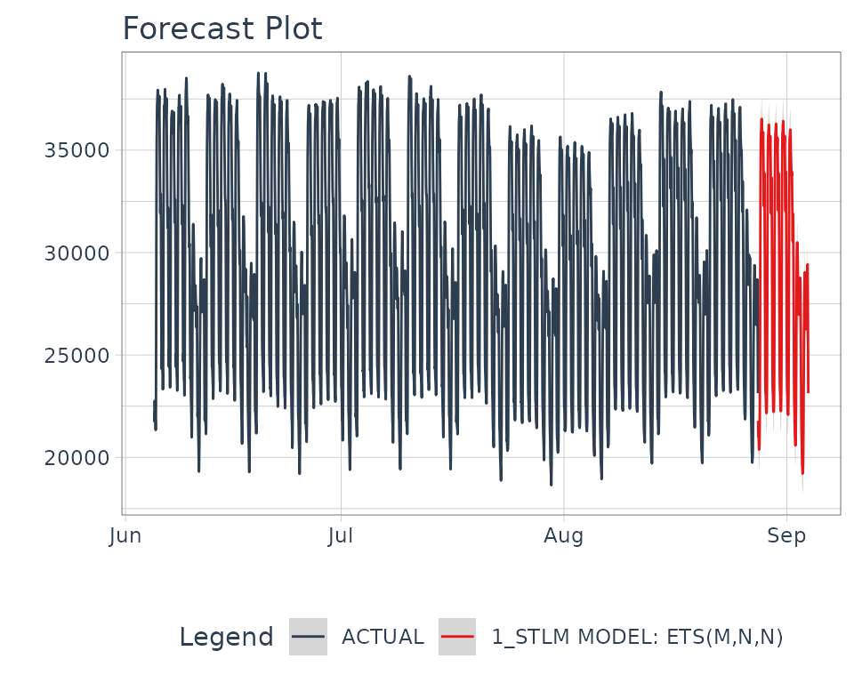

And now you’ve just created a new model. Just wrap it up in a package and you’ve extended parsnip and modeltime. Congrats!

Further Resources

I’d recommend looking at the code for parsnip-arima_reg.R and parsnip-arima_reg_data.R to see how this process is implemented inside a package.