Visualize Anomalies for One or More Time Series

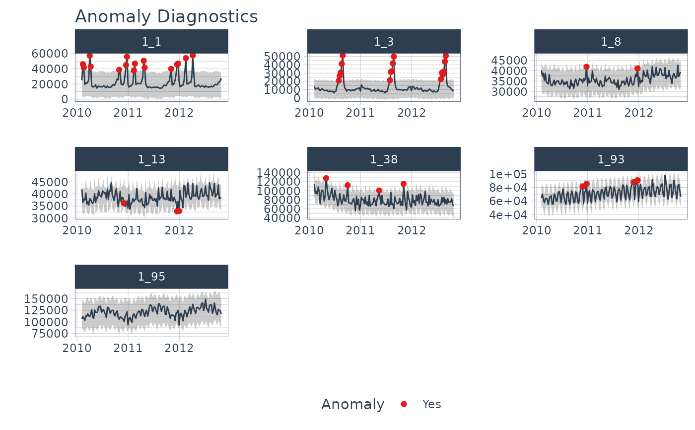
An interactive and scalable function for visualizing anomalies in time series data. Plots are available in interactive plotly (default) and static ggplot2 format.

Usage

plot_anomaly_diagnostics(
  .data,
  .date_var,
  .value,
  .facet_vars = NULL,
  .frequency = "auto",
  .trend = "auto",
  .alpha = 0.05,
  .max_anomalies = 0.2,
  .message = TRUE,
  .facet_ncol = 1,
  .facet_nrow = 1,
  .facet_scales = "free",
  .facet_dir = "h",
  .facet_collapse = FALSE,
  .facet_collapse_sep = " ",
  .facet_strip_remove = FALSE,
  .line_color = "#2c3e50",
  .line_size = 0.5,
  .line_type = 1,
  .line_alpha = 1,
  .anom_color = "#e31a1c",
  .anom_alpha = 1,
  .anom_size = 1.5,
  .ribbon_fill = "grey20",
  .ribbon_alpha = 0.2,
  .legend_show = TRUE,
  .title = "Anomaly Diagnostics",
  .x_lab = "",
  .y_lab = "",
  .color_lab = "Anomaly",
  .interactive = TRUE,
  .trelliscope = FALSE,
  .trelliscope_params = list()
)

Arguments

.data

A tibble or data.frame with a time-based column

.date_var

A column containing either date or date-time values

.value

A column containing numeric values

.facet_vars

One or more grouping columns that broken out into ggplot2 facets. These can be selected using tidyselect() helpers (e.g contains()).

.frequency

Controls the seasonal adjustment (removal of seasonality). Input can be either "auto", a time-based definition (e.g. "2 weeks"), or a numeric number of observations per frequency (e.g. 10). Refer to tk_get_frequency().

.trend

Controls the trend component. For STL, trend controls the sensitivity of the LOESS smoother, which is used to remove the remainder. Refer to tk_get_trend().

.alpha

Controls the width of the "normal" range. Lower values are more conservative while higher values are less prone to incorrectly classifying "normal" observations.

.max_anomalies

The maximum percent of anomalies permitted to be identified.

.message

A boolean. If TRUE, will output information related to automatic frequency and trend selection (if applicable).

.facet_ncol

Number of facet columns.

.facet_nrow

Number of facet rows (only used for .trelliscope = TRUE)

.facet_scales

Control facet x & y-axis ranges. Options include "fixed", "free", "free_y", "free_x"

.facet_dir

The direction of faceting ("h" for horizontal, "v" for vertical). Default is "h".

.facet_collapse

Multiple facets included on one facet strip instead of multiple facet strips.

.facet_collapse_sep

The separator used for collapsing facets.

.facet_strip_remove

Whether or not to remove the strip and text label for each facet.

.line_color

Line color.

.line_size

Line size.

.line_type

Line type.

.line_alpha

Line alpha (opacity). Range: (0, 1).

.anom_color

Color for the anomaly dots

.anom_alpha

Opacity for the anomaly dots. Range: (0, 1).

.anom_size

Size for the anomaly dots

.ribbon_fill

Fill color for the acceptable range

.ribbon_alpha

Fill opacity for the acceptable range. Range: (0, 1).

.legend_show

Toggles on/off the Legend

.title

Plot title.

.x_lab

Plot x-axis label

.y_lab

Plot y-axis label

.color_lab

Plot label for the color legend

.interactive

If TRUE, returns a plotly interactive plot. If FALSE, returns a static ggplot2 plot.

.trelliscope

Returns either a normal plot or a trelliscopejs plot (great for many time series) Must have trelliscopejs installed.

.trelliscope_params

Pass parameters to the trelliscopejs::facet_trelliscope() function as a list(). The only parameters that cannot be passed are:

ncol: use .facet_ncol
nrow: use .facet_nrow
scales: use facet_scales
as_plotly: use .interactive

Value

A plotly or ggplot2 visualization

Details

The plot_anomaly_diagnostics() is a visualization wrapper for tk_anomaly_diagnostics() group-wise anomaly detection, implements a 2-step process to detect outliers in time series.

Step 1: Detrend & Remove Seasonality using STL Decomposition

The decomposition separates the "season" and "trend" components from the "observed" values leaving the "remainder" for anomaly detection.

The user can control two parameters: frequency and trend.

.frequency: Adjusts the "season" component that is removed from the "observed" values.
.trend: Adjusts the trend window (t.window parameter from stats::stl() that is used.

The user may supply both .frequency and .trend as time-based durations (e.g. "6 weeks") or numeric values (e.g. 180) or "auto", which predetermines the frequency and/or trend based on the scale of the time series using the tk_time_scale_template().

Step 2: Anomaly Detection

Once "trend" and "season" (seasonality) is removed, anomaly detection is performed on the "remainder". Anomalies are identified, and boundaries (recomposed_l1 and recomposed_l2) are determined.

The Anomaly Detection Method uses an inner quartile range (IQR) of +/-25 the median.

IQR Adjustment, alpha parameter

With the default alpha = 0.05, the limits are established by expanding the 25/75 baseline by an IQR Factor of 3 (3X). The IQR Factor = 0.15 / alpha (hence 3X with alpha = 0.05):

To increase the IQR Factor controlling the limits, decrease the alpha, which makes it more difficult to be an outlier.
Increase alpha to make it easier to be an outlier.
The IQR outlier detection method is used in forecast::tsoutliers().
A similar outlier detection method is used by Twitter's AnomalyDetection package.
Both Twitter and Forecast tsoutliers methods have been implemented in Business Science's anomalize package.

References

CLEVELAND, R. B., CLEVELAND, W. S., MCRAE, J. E., AND TERPENNING, I. STL: A Seasonal-Trend Decomposition Procedure Based on Loess. Journal of Official Statistics, Vol. 6, No. 1 (1990), pp. 3-73.
Owen S. Vallis, Jordan Hochenbaum and Arun Kejariwal (2014). A Novel Technique for Long-Term Anomaly Detection in the Cloud. Twitter Inc.

Examples

library(dplyr)

walmart_sales_weekly %>%
    group_by(id) %>%
    plot_anomaly_diagnostics(Date, Weekly_Sales,
                             .message = FALSE,
                             .facet_ncol = 3,
                             .ribbon_alpha = 0.25,
                             .interactive = FALSE)