Mutate (for Time Series Data)

mutate_by_time() is a time-based variant of the popular dplyr::mutate() function that uses .date_var to specify a date or date-time column and .by to group the calculation by groups like "5 seconds", "week", or "3 months".

Usage

mutate_by_time(
  .data,
  .date_var,
  .by = "day",
  ...,
  .type = c("floor", "ceiling", "round")
)

Arguments

.data

A tbl object or data.frame

.date_var

A column containing date or date-time values to summarize. If missing, attempts to auto-detect date column.

.by

A time unit to summarise by. Time units are collapsed using lubridate::floor_date() or lubridate::ceiling_date().

The value can be:

• second

• minute

• hour

• day

• week

• month

• bimonth

• quarter

• season

• halfyear

• year

Arbitrary unique English abbreviations as in the lubridate::period() constructor are allowed.

...

Name-value pairs. The name gives the name of the column in the output.

The value can be:

• A vector of length 1, which will be recycled to the correct length.

• A vector the same length as the current group (or the whole data frame if ungrouped).

• NULL, to remove the column.

• A data frame or tibble, to create multiple columns in the output.

.type

One of "floor", "ceiling", or "round. Defaults to "floor". See lubridate::round_date.

Value

A tibble or data.frame

See also

Time-Based dplyr functions:

• summarise_by_time() - Easily summarise using a date column.

• mutate_by_time() - Simplifies applying mutations by time windows.

• pad_by_time() - Insert time series rows with regularly spaced timestamps

• filter_by_time() - Quickly filter using date ranges.

• filter_period() - Apply filtering expressions inside periods (windows)

• slice_period() - Apply slice inside periods (windows)

• condense_period() - Convert to a different periodicity

• between_time() - Range detection for date or date-time sequences.

• slidify() - Turn any function into a sliding (rolling) function

Examples

# Libraries
library(dplyr)

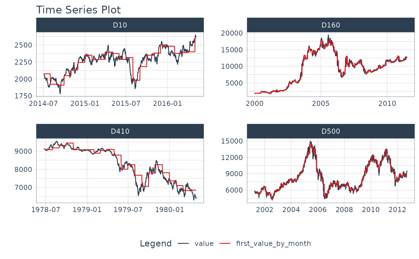
# First value in each month
m4_daily_first_by_month_tbl <- m4_daily %>%
    group_by(id) %>%
    mutate_by_time(
        .date_var = date,
        .by       = "month", # Setup for monthly aggregation
        # mutate recycles a single value
        first_value_by_month  = first(value)
    )
m4_daily_first_by_month_tbl
#> # A tibble: 9,743 × 4
#> # Groups:   id [4]
#>    id    date       value first_value_by_month
#>    <fct> <date>     <dbl>                <dbl>
#>  1 D10   2014-07-03 2076.                2076.
#>  2 D10   2014-07-04 2073.                2076.
#>  3 D10   2014-07-05 2049.                2076.
#>  4 D10   2014-07-06 2049.                2076.
#>  5 D10   2014-07-07 2006.                2076.
#>  6 D10   2014-07-08 2018.                2076.
#>  7 D10   2014-07-09 2019.                2076.
#>  8 D10   2014-07-10 2007.                2076.
#>  9 D10   2014-07-11 2010                 2076.
#> 10 D10   2014-07-12 2002.                2076.
#> # ℹ 9,733 more rows

# Visualize Time Series vs 1st Value Each Month
m4_daily_first_by_month_tbl %>%
    tidyr::pivot_longer(value:first_value_by_month) %>%
    plot_time_series(date, value, name,
                     .facet_scale = "free", .facet_ncol = 2,
                     .smooth = FALSE, .interactive = FALSE)