Visualize a Time Series Linear Regression Formula

A wrapper for stats::lm() that overlays a linear regression fitted model over a time series, which can help show the effect of feature engineering

Usage

plot_time_series_regression(
  .data,
  .date_var,
  .formula,
  .show_summary = FALSE,
  ...
)

Arguments

.data

A tibble or data.frame with a time-based column

.date_var

A column containing either date or date-time values

.formula

A linear regression formula. The left-hand side of the formula is used as the y-axis value. The right-hand side of the formula is used to develop the linear regression model. See stats::lm() for details.

.show_summary

If TRUE, prints the summary.lm().

...

Additional arguments passed to plot_time_series()

Value

A static ggplot2 plot or an interactive plotly plot

Details

plot_time_series_regression() is a scalable function that works with both ungrouped and grouped data.frame objects (and tibbles!).

Time Series Formula

The .formula uses stats::lm() to apply a linear regression, which is used to visualize the effect of feature engineering on a time series.

• The left-hand side of the formula is used as the y-axis value.

• The right-hand side of the formula is used to develop the linear regression model.

Interactive by Default

plot_time_series_regression() is built for exploration using:

• Interactive Plots: plotly (default) - Great for exploring!

• Static Plots: ggplot2 (set .interactive = FALSE) - Great for PDF Reports

By default, an interactive plotly visualization is returned.

Scalable with Facets & Dplyr Groups

plot_time_series_regression() returns multiple time series plots using ggplot2 facets:

• group_by() - If groups are detected, multiple facets are returned

• plot_time_series_regression(.facet_vars) - You can manually supply facets as well.

Examples

library(dplyr)
library(lubridate)

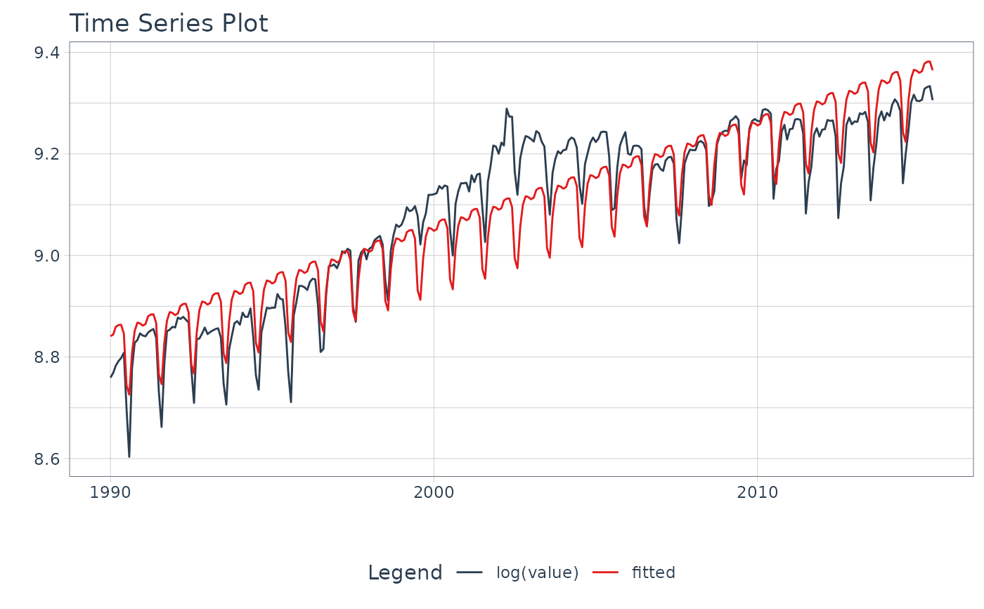
# ---- SINGLE SERIES ----
m4_monthly %>%
    filter(id == "M750") %>%
    plot_time_series_regression(
        .date_var     = date,
        .formula      = log(value) ~ as.numeric(date) + month(date, label = TRUE),
        .show_summary = TRUE,
        .facet_ncol   = 2,
        .interactive  = FALSE
    )
#> 
#> Call:
#> stats::lm(formula = .formula, data = df)
#> 
#> Residuals:
#>      Min       1Q   Median       3Q      Max 
#> -0.12770 -0.05159 -0.01753  0.05142  0.17828 
#> 
#> Coefficients:
#>                                Estimate Std. Error t value Pr(>|t|)    
#> (Intercept)                   8.407e+00  1.651e-02 509.199  < 2e-16 ***
#> as.numeric(date)              5.679e-05  1.348e-06  42.118  < 2e-16 ***
#> month(date, label = TRUE).L  -3.584e-02  1.256e-02  -2.854 0.004625 ** 
#> month(date, label = TRUE).Q   7.509e-02  1.256e-02   5.979 6.51e-09 ***
#> month(date, label = TRUE).C   7.879e-02  1.256e-02   6.273 1.27e-09 ***
#> month(date, label = TRUE)^4  -4.931e-02  1.256e-02  -3.926 0.000108 ***
#> month(date, label = TRUE)^5  -7.964e-02  1.256e-02  -6.341 8.61e-10 ***
#> month(date, label = TRUE)^6   1.215e-02  1.256e-02   0.967 0.334270    
#> month(date, label = TRUE)^7   5.196e-02  1.256e-02   4.137 4.60e-05 ***
#> month(date, label = TRUE)^8   1.200e-02  1.256e-02   0.955 0.340143    
#> month(date, label = TRUE)^9  -3.433e-02  1.256e-02  -2.733 0.006652 ** 
#> month(date, label = TRUE)^10 -1.566e-02  1.256e-02  -1.247 0.213483    
#> month(date, label = TRUE)^11  1.182e-02  1.256e-02   0.941 0.347375    
#> ---
#> Signif. codes:  0 ‘***’ 0.001 ‘**’ 0.01 ‘*’ 0.05 ‘.’ 0.1 ‘ ’ 1
#> 
#> Residual standard error: 0.06341 on 293 degrees of freedom
#> Multiple R-squared:  0.8695,	Adjusted R-squared:  0.8641 
#> F-statistic: 162.6 on 12 and 293 DF,  p-value: < 2.2e-16
#> 



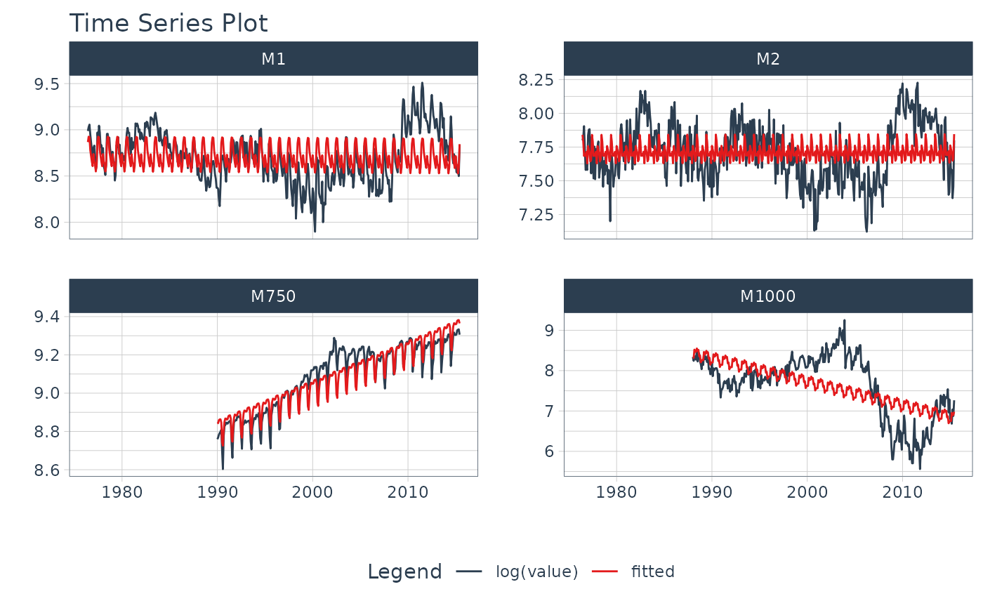
# ---- GROUPED SERIES ----
m4_monthly %>%
    group_by(id) %>%
    plot_time_series_regression(
        .date_var    = date,
        .formula     = log(value) ~ as.numeric(date) + month(date, label = TRUE),
        .facet_ncol  = 2,
        .interactive = FALSE
    )