Scaling and Modeling with tidyquant

Designed for the data science workflow of the tidyverse

Overview

The greatest benefit to tidyquant is the ability to apply the data science workflow to easily model and scale your financial analysis as described in R for Data Science. Scaling is the process of creating an analysis for one asset and then extending it to multiple groups. This idea of scaling is incredibly useful to financial analysts because typically one wants to compare many assets to make informed decisions. Fortunately, the tidyquant package integrates with the tidyverse making scaling super simple!

All tidyquant functions return data in the tibble (tidy data frame) format, which allows for interaction within the tidyverse. This means we can:

Seamlessly scale data retrieval and mutations
Use the pipe (%>%) for chaining operations
Use dplyr and tidyr: select, filter, group_by, nest/unnest, spread/gather, etc
Use purrr: mapping functions with map()
Model financial analysis using the data science workflow in R for Data Science

We’ll go through some useful techniques for getting and manipulating groups of data.

Prerequisites

Load the tidyquant package to get started.

# Loads tidyquant, xts, quantmod, TTR, and PerformanceAnalytics
library(tidyverse)
library(tidyquant)

1.0 Scaling the Getting of Financial Data

A very basic example is retrieving the stock prices for multiple stocks. There are three primary ways to do this:

Method 1: Map a character vector with multiple stock symbols

c("AAPL", "GOOG", "META") %>%
    tq_get(get = "stock.prices", from = "2016-01-01", to = "2017-01-01")

## # A tibble: 756 × 8
##    symbol date        open  high   low close    volume adjusted
##    <chr>  <date>     <dbl> <dbl> <dbl> <dbl>     <dbl>    <dbl>
##  1 AAPL   2016-01-04  25.7  26.3  25.5  26.3 270597600     23.9
##  2 AAPL   2016-01-05  26.4  26.5  25.6  25.7 223164000     23.3
##  3 AAPL   2016-01-06  25.1  25.6  25.0  25.2 273829600     22.9
##  4 AAPL   2016-01-07  24.7  25.0  24.1  24.1 324377600     21.9
##  5 AAPL   2016-01-08  24.6  24.8  24.2  24.2 283192000     22.0
##  6 AAPL   2016-01-11  24.7  24.8  24.3  24.6 198957600     22.4
##  7 AAPL   2016-01-12  25.1  25.2  24.7  25.0 196616800     22.7
##  8 AAPL   2016-01-13  25.1  25.3  24.3  24.3 249758400     22.1
##  9 AAPL   2016-01-14  24.5  25.1  23.9  24.9 252680400     22.6
## 10 AAPL   2016-01-15  24.0  24.4  23.8  24.3 319335600     22.1
## # ℹ 746 more rows

The output is a single level tibble with all or the stock prices in one tibble. The auto-generated column name is “symbol”, which can be preemptively renamed by giving the vector a name (e.g. stocks <- c("AAPL", "GOOG", "META")) and then piping to tq_get.

Method 2: Map a tibble with stocks in first column

First, get a stock list in data frame format either by making the tibble or retrieving from tq_index / tq_exchange. The stock symbols must be in the first column.

Method 2A: Make a tibble

stock_list <- tibble(stocks = c("AAPL", "JPM", "CVX"),
                     industry = c("Technology", "Financial", "Energy"))
stock_list

## # A tibble: 3 × 2
##   stocks industry  
##   <chr>  <chr>     
## 1 AAPL   Technology
## 2 JPM    Financial 
## 3 CVX    Energy

Second, send the stock list to tq_get. Notice how the symbol and industry columns are automatically expanded the length of the stock prices.

stock_list %>%
    tq_get(get = "stock.prices", from = "2016-01-01", to = "2017-01-01")

## # A tibble: 756 × 9
##    stocks industry   date        open  high   low close    volume adjusted
##    <chr>  <chr>      <date>     <dbl> <dbl> <dbl> <dbl>     <dbl>    <dbl>
##  1 AAPL   Technology 2016-01-04  25.7  26.3  25.5  26.3 270597600     23.9
##  2 AAPL   Technology 2016-01-05  26.4  26.5  25.6  25.7 223164000     23.3
##  3 AAPL   Technology 2016-01-06  25.1  25.6  25.0  25.2 273829600     22.9
##  4 AAPL   Technology 2016-01-07  24.7  25.0  24.1  24.1 324377600     21.9
##  5 AAPL   Technology 2016-01-08  24.6  24.8  24.2  24.2 283192000     22.0
##  6 AAPL   Technology 2016-01-11  24.7  24.8  24.3  24.6 198957600     22.4
##  7 AAPL   Technology 2016-01-12  25.1  25.2  24.7  25.0 196616800     22.7
##  8 AAPL   Technology 2016-01-13  25.1  25.3  24.3  24.3 249758400     22.1
##  9 AAPL   Technology 2016-01-14  24.5  25.1  23.9  24.9 252680400     22.6
## 10 AAPL   Technology 2016-01-15  24.0  24.4  23.8  24.3 319335600     22.1
## # ℹ 746 more rows

Method 2B: Use index or exchange

Get an index…

tq_index("DOW")

## # A tibble: 31 × 8
##    symbol company      identifier sedol weight sector shares_held local_currency
##    <chr>  <chr>        <chr>      <chr>  <dbl> <chr>        <dbl> <chr>         
##  1 UNH    UNITEDHEALT… 91324P102  2917… 0.0811 -          5654065 USD           
##  2 MSFT   MICROSOFT C… 594918104  2588… 0.0693 -          5654065 USD           
##  3 GS     GOLDMAN SAC… 38141G104  2407… 0.0683 -          5654065 USD           
##  4 HD     HOME DEPOT … 437076102  2434… 0.0634 -          5654065 USD           
##  5 CAT    CATERPILLAR… 149123101  2180… 0.0599 -          5654065 USD           
##  6 CRM    SALESFORCE … 79466L302  2310… 0.0495 -          5654065 USD           
##  7 AMGN   AMGEN INC    031162100  2023… 0.0471 -          5654065 USD           
##  8 MCD    MCDONALD S … 580135101  2550… 0.0464 -          5654065 USD           
##  9 V      VISA INC CL… 92826C839  B2PZ… 0.0459 -          5654065 USD           
## 10 TRV    TRAVELERS C… 89417E109  2769… 0.0376 -          5654065 USD           
## # ℹ 21 more rows

…or, get an exchange.

tq_exchange("NYSE")

Send the index or exchange to tq_get. Important Note: This can take several minutes depending on the size of the index or exchange, which is why only the first three stocks are evaluated in the vignette.

tq_index("DOW") %>%
    slice(1:3) %>%
    tq_get(get = "stock.prices")

## # A tibble: 7,731 × 15
##    symbol company      identifier sedol weight sector shares_held local_currency
##    <chr>  <chr>        <chr>      <chr>  <dbl> <chr>        <dbl> <chr>         
##  1 UNH    UNITEDHEALT… 91324P102  2917… 0.0811 -          5654065 USD           
##  2 UNH    UNITEDHEALT… 91324P102  2917… 0.0811 -          5654065 USD           
##  3 UNH    UNITEDHEALT… 91324P102  2917… 0.0811 -          5654065 USD           
##  4 UNH    UNITEDHEALT… 91324P102  2917… 0.0811 -          5654065 USD           
##  5 UNH    UNITEDHEALT… 91324P102  2917… 0.0811 -          5654065 USD           
##  6 UNH    UNITEDHEALT… 91324P102  2917… 0.0811 -          5654065 USD           
##  7 UNH    UNITEDHEALT… 91324P102  2917… 0.0811 -          5654065 USD           
##  8 UNH    UNITEDHEALT… 91324P102  2917… 0.0811 -          5654065 USD           
##  9 UNH    UNITEDHEALT… 91324P102  2917… 0.0811 -          5654065 USD           
## 10 UNH    UNITEDHEALT… 91324P102  2917… 0.0811 -          5654065 USD           
## # ℹ 7,721 more rows
## # ℹ 7 more variables: date <date>, open <dbl>, high <dbl>, low <dbl>,
## #   close <dbl>, volume <dbl>, adjusted <dbl>

You can use any applicable “getter” to get data for every stock in an index or an exchange! This includes: “stock.prices”, “key.ratios”, “key.stats”, and more.

2.0 Scaling the Mutation of Financial Data

Once you get the data, you typically want to do something with it. You can easily do this at scale. Let’s get the yearly returns for multiple stocks using tq_transmute. First, get the prices. We’ll use the FANG data set, but you typically will use tq_get to retrieve data in “tibble” format.

FANG

## # A tibble: 4,032 × 8
##    symbol date        open  high   low close    volume adjusted
##    <chr>  <date>     <dbl> <dbl> <dbl> <dbl>     <dbl>    <dbl>
##  1 META   2013-01-02  27.4  28.2  27.4  28    69846400     28  
##  2 META   2013-01-03  27.9  28.5  27.6  27.8  63140600     27.8
##  3 META   2013-01-04  28.0  28.9  27.8  28.8  72715400     28.8
##  4 META   2013-01-07  28.7  29.8  28.6  29.4  83781800     29.4
##  5 META   2013-01-08  29.5  29.6  28.9  29.1  45871300     29.1
##  6 META   2013-01-09  29.7  30.6  29.5  30.6 104787700     30.6
##  7 META   2013-01-10  30.6  31.5  30.3  31.3  95316400     31.3
##  8 META   2013-01-11  31.3  32.0  31.1  31.7  89598000     31.7
##  9 META   2013-01-14  32.1  32.2  30.6  31.0  98892800     31.0
## 10 META   2013-01-15  30.6  31.7  29.9  30.1 173242600     30.1
## # ℹ 4,022 more rows

Second, use group_by to group by stock symbol. Third, apply the mutation. We can do this in one easy workflow. The periodReturn function is applied to each group of stock prices, and a new data frame was returned with the annual returns in the correct periodicity.

FANG_returns_yearly <- FANG %>%
    group_by(symbol) %>%
    tq_transmute(select     = adjusted, 
                 mutate_fun = periodReturn, 
                 period     = "yearly", 
                 col_rename = "yearly.returns")

Last, we can visualize the returns.

FANG_returns_yearly %>%
    ggplot(aes(x = year(date), y = yearly.returns, fill = symbol)) +
    geom_bar(position = "dodge", stat = "identity") +
    labs(title = "FANG: Annual Returns", 
         subtitle = "Mutating at scale is quick and easy!",
         y = "Returns", x = "", color = "") +
    scale_y_continuous(labels = scales::percent) +
    coord_flip() +
    theme_tq() +
    scale_fill_tq()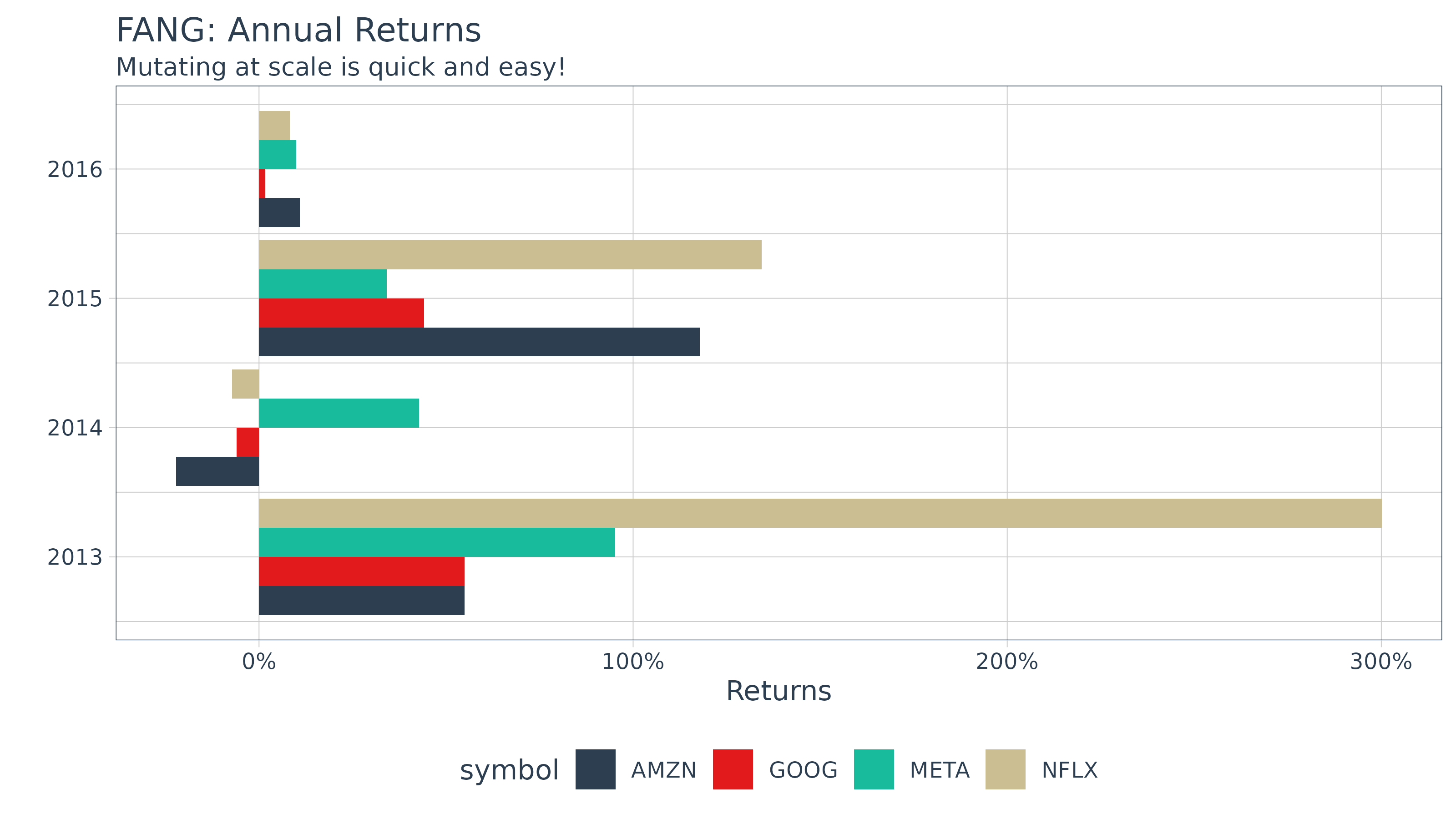

3.0 Modeling Financial Data using purrr

Eventually you will want to begin modeling (or more generally applying functions) at scale! One of the best features of the tidyverse is the ability to map functions to nested tibbles using purrr. From the Many Models chapter of “R for Data Science”, we can apply the same modeling workflow to financial analysis. Using a two step workflow:

Model a single stock
Scale to many stocks

Let’s go through an example to illustrate.

Example: Applying a Regression Model to Detect a Positive Trend

In this example, we’ll use a simple linear model to identify the trend in annual returns to determine if the stock returns are decreasing or increasing over time.

Analyze a Single Stock

First, let’s collect stock data with tq_get()

AAPL <- tq_get("AAPL", from = "2007-01-01", to = "2016-12-31")
AAPL

## # A tibble: 2,518 × 8
##    symbol date        open  high   low close     volume adjusted
##    <chr>  <date>     <dbl> <dbl> <dbl> <dbl>      <dbl>    <dbl>
##  1 AAPL   2007-01-03  3.08  3.09  2.92  2.99 1238319600     2.53
##  2 AAPL   2007-01-04  3.00  3.07  2.99  3.06  847260400     2.59
##  3 AAPL   2007-01-05  3.06  3.08  3.01  3.04  834741600     2.57
##  4 AAPL   2007-01-08  3.07  3.09  3.05  3.05  797106800     2.58
##  5 AAPL   2007-01-09  3.09  3.32  3.04  3.31 3349298400     2.80
##  6 AAPL   2007-01-10  3.38  3.49  3.34  3.46 2952880000     2.93
##  7 AAPL   2007-01-11  3.43  3.46  3.40  3.42 1440252800     2.90
##  8 AAPL   2007-01-12  3.38  3.39  3.33  3.38 1312690400     2.86
##  9 AAPL   2007-01-16  3.42  3.47  3.41  3.47 1244076400     2.94
## 10 AAPL   2007-01-17  3.48  3.49  3.39  3.39 1646260000     2.87
## # ℹ 2,508 more rows

Next, come up with a function to help us collect annual log returns. The function below mutates the stock prices to period returns using tq_transmute(). We add the type = "log" and period = "monthly" arguments to ensure we retrieve a tibble of monthly log returns. Last, we take the mean of the monthly returns to get MMLR.

get_annual_returns <- function(stock.returns) {
    stock.returns %>%
        tq_transmute(select     = adjusted, 
                     mutate_fun = periodReturn, 
                     type       = "log", 
                     period     = "yearly")
}

Let’s test get_annual_returns out. We now have the annual log returns over the past ten years.

AAPL_annual_log_returns <- get_annual_returns(AAPL)
AAPL_annual_log_returns

## # A tibble: 10 × 2
##    date       yearly.returns
##    <date>              <dbl>
##  1 2007-12-31         0.860 
##  2 2008-12-31        -0.842 
##  3 2009-12-31         0.904 
##  4 2010-12-31         0.426 
##  5 2011-12-30         0.228 
##  6 2012-12-31         0.282 
##  7 2013-12-31         0.0776
##  8 2014-12-31         0.341 
##  9 2015-12-31        -0.0306
## 10 2016-12-30         0.118

Let’s visualize to identify trends. We can see from the linear trend line that AAPL’s stock returns are declining.

AAPL_annual_log_returns %>%
    ggplot(aes(x = year(date), y = yearly.returns)) + 
    geom_hline(yintercept = 0, color = palette_light()[[1]]) +
    geom_point(size = 2, color = palette_light()[[3]]) +
    geom_line(linewidth = 1, color = palette_light()[[3]]) + 
    geom_smooth(method = "lm", se = FALSE) +
    labs(title = "AAPL: Visualizing Trends in Annual Returns",
         x = "", y = "Annual Returns", color = "") +
    theme_tq()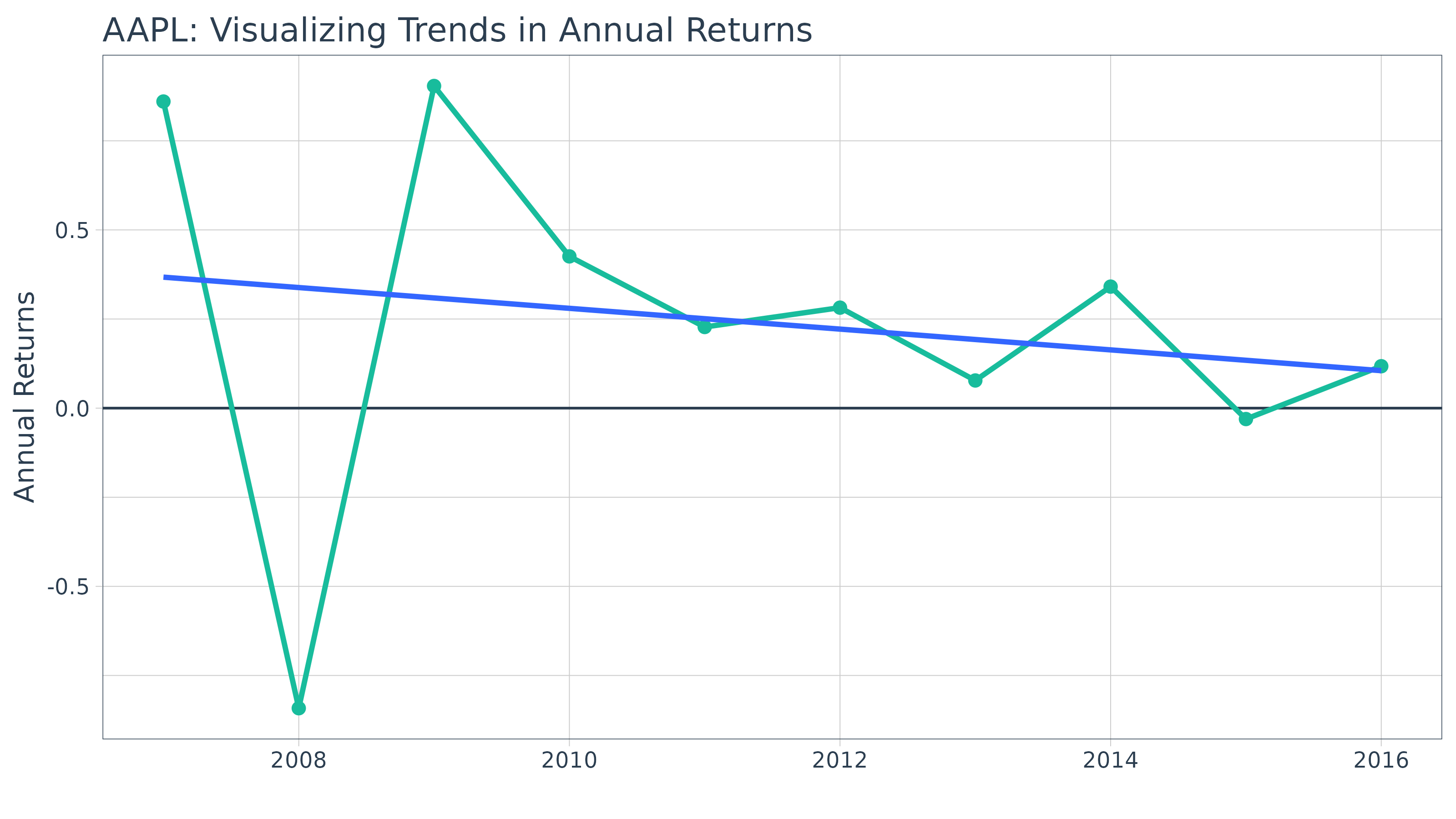

Now, we can get the linear model using the lm() function. However, there is one problem: the output is not “tidy”.

mod <- lm(yearly.returns ~ year(date), data = AAPL_annual_log_returns)
mod

## 
## Call:
## lm(formula = yearly.returns ~ year(date), data = AAPL_annual_log_returns)
## 
## Coefficients:
## (Intercept)   year(date)  
##    58.86284     -0.02915

We can utilize the broom package to get “tidy” data from the model. There’s three primary functions:

augment: adds columns to the original data such as predictions, residuals and cluster assignments
glance: provides a one-row summary of model-level statistics
tidy: summarizes a model’s statistical findings such as coefficients of a regression

We’ll use tidy to retrieve the model coefficients.

library(broom)
tidy(mod)

## # A tibble: 2 × 5
##   term        estimate std.error statistic p.value
##   <chr>          <dbl>     <dbl>     <dbl>   <dbl>
## 1 (Intercept)  58.9     113.         0.520   0.617
## 2 year(date)   -0.0291    0.0562    -0.518   0.618

Adding to our workflow, we have the following:

get_model <- function(stock_data) {
    annual_returns <- get_annual_returns(stock_data)
    mod <- lm(yearly.returns ~ year(date), data = annual_returns)
    tidy(mod)
}

Testing it out on a single stock. We can see that the “term” that contains the direction of the trend (the slope) is “year(date)”. The interpretation is that as year increases one unit, the annual returns decrease by 3%.

get_model(AAPL)

## # A tibble: 2 × 5
##   term        estimate std.error statistic p.value
##   <chr>          <dbl>     <dbl>     <dbl>   <dbl>
## 1 (Intercept)  58.9     113.         0.520   0.617
## 2 year(date)   -0.0291    0.0562    -0.518   0.618

Now that we have identified the trend direction, it looks like we are ready to scale.

Scale to Many Stocks

Once the analysis for one stock is done scale to many stocks is simple. For brevity, we’ll randomly sample ten stocks from the S&P500 with a call to dplyr::sample_n().

set.seed(10)
stocks_tbl <- tq_index("SP500") %>%
    sample_n(5) 
stocks_tbl

## # A tibble: 5 × 8
##   symbol company      identifier sedol  weight sector shares_held local_currency
##   <chr>  <chr>        <chr>      <chr>   <dbl> <chr>        <dbl> <chr>         
## 1 GNRC   GENERAC HOL… 368736104  B619… 1.73e-4 -           746285 USD           
## 2 NOC    NORTHROP GR… 666807102  2648… 1.53e-3 -          1722557 USD           
## 3 HUBB   HUBBELL INC  443510607  BDFG… 5.02e-4 -           651644 USD           
## 4 STX    SEAGATE TEC… G7997R103  BKVD… 4.14e-4 -          2349510 USD           
## 5 INCY   INCYTE CORP  45337C102  2471… 2.41e-4 -          2262477 USD

We can now apply our analysis function to the stocks using dplyr::mutate() and purrr::map(). The mutate() function adds a column to our tibble, and the map() function maps our custom get_model function to our tibble of stocks using the symbol column. The tidyr::unnest() function unrolls the nested data frame so all of the model statistics are accessible in the top data frame level. The filter, arrange and select steps just manipulate the data frame to isolate and arrange the data for our viewing.

stocks_model_stats <- stocks_tbl %>%
    select(symbol, company) %>%
    tq_get(from = "2007-01-01", to = "2016-12-31") %>%
    
    # Nest 
    group_by(symbol, company) %>%
    nest() %>%
    
    # Apply the get_model() function to the new "nested" data column
    mutate(model = map(data, get_model)) %>%
    
    # Unnest and collect slope
    unnest(model) %>%
    filter(term == "year(date)") %>%
    arrange(desc(estimate)) %>%
    select(-term)

stocks_model_stats

## # A tibble: 5 × 7
## # Groups:   symbol, company [5]
##   symbol company                   data     estimate std.error statistic p.value
##   <chr>  <chr>                     <list>      <dbl>     <dbl>     <dbl>   <dbl>
## 1 NOC    NORTHROP GRUMMAN CORP     <tibble>  0.0456     0.0280     1.63    0.142
## 2 STX    SEAGATE TECHNOLOGY HOLDI… <tibble>  0.0381     0.0958     0.398   0.701
## 3 INCY   INCYTE CORP               <tibble>  0.0210     0.0682     0.308   0.766
## 4 HUBB   HUBBELL INC               <tibble>  0.00574    0.0270     0.213   0.837
## 5 GNRC   GENERAC HOLDINGS INC      <tibble> -0.0870     0.0741    -1.17    0.293

We’re done! We now have the coefficient of the linear regression that tracks the direction of the trend line. We can easily extend this type of analysis to larger lists or stock indexes. For example, the entire S&P500 could be analyzed removing the sample_n() following the call to tq_index("SP500").

4.0 Error Handling when Scaling

Eventually you will run into a stock index, stock symbol, FRED data code, etc that cannot be retrieved. Possible reasons are:

An index becomes out of date
A company goes private
A stock ticker symbol changes
Yahoo / FRED just doesn’t like your stock symbol / FRED code

This becomes painful when scaling if the functions return errors. So, the tq_get() function is designed to handle errors gracefully. What this means is an NA value is returned when an error is generated along with a gentle error warning.

tq_get("XYZ", "stock.prices")

## [1] NA

Pros and Cons to Built-In Error-Handling

There are pros and cons to this approach that you may not agree with, but I believe helps in the long run. Just be aware of what happens:

Pros: Long running scripts are not interrupted because of one error
Cons: Errors can be inadvertently handled or flow downstream if the user does not read the warnings

Bad Apples Fail Gracefully, tq_get

Let’s see an example when using tq_get() to get the stock prices for a long list of stocks with one BAD APPLE. The argument complete_cases comes in handy. The default is TRUE, which removes “bad apples” so future analysis have complete cases to compute on. Note that a gentle warning stating that an error occurred and was dealt with by removing the rows from the results.

c("AAPL", "GOOG", "BAD APPLE") %>%
    tq_get(get = "stock.prices", complete_cases = TRUE)

## Warning: There was 1 warning in `dplyr::mutate()`.
## ℹ In argument: `data.. = purrr::map(...)`.
## Caused by warning:
## ! x = 'BAD APPLE', get = 'stock.prices': Error in getSymbols.yahoo(Symbols = "BAD APPLE", env = <environment>, : Unable to import "BAD APPLE".
## URL using bad/illegal format or missing URL
##  Removing BAD APPLE.

## # A tibble: 5,096 × 8
##    symbol date        open  high   low close    volume adjusted
##    <chr>  <date>     <dbl> <dbl> <dbl> <dbl>     <dbl>    <dbl>
##  1 AAPL   2014-01-02  19.8  19.9  19.7  19.8 234684800     17.3
##  2 AAPL   2014-01-03  19.7  19.8  19.3  19.3 392467600     16.9
##  3 AAPL   2014-01-06  19.2  19.5  19.1  19.4 412610800     17.0
##  4 AAPL   2014-01-07  19.4  19.5  19.2  19.3 317209200     16.9
##  5 AAPL   2014-01-08  19.2  19.5  19.2  19.4 258529600     17.0
##  6 AAPL   2014-01-09  19.5  19.5  19.1  19.2 279148800     16.8
##  7 AAPL   2014-01-10  19.3  19.3  19.0  19.0 304976000     16.7
##  8 AAPL   2014-01-13  18.9  19.4  18.9  19.1 378492800     16.8
##  9 AAPL   2014-01-14  19.2  19.5  19.2  19.5 332561600     17.1
## 10 AAPL   2014-01-15  19.8  20.0  19.7  19.9 391638800     17.4
## # ℹ 5,086 more rows

Now switching complete_cases = FALSE will retain any errors as NA values in a nested data frame. Notice that the error message and output change. The error message now states that the NA values exist in the output and the return is a “nested” data structure.

c("AAPL", "GOOG", "BAD APPLE") %>%
    tq_get(get = "stock.prices", complete_cases = FALSE)

## Warning: There was 1 warning in `dplyr::mutate()`.
## ℹ In argument: `data.. = purrr::map(...)`.
## Caused by warning:
## ! x = 'BAD APPLE', get = 'stock.prices': Error in getSymbols.yahoo(Symbols = "BAD APPLE", env = <environment>, : Unable to import "BAD APPLE".
## URL using bad/illegal format or missing URL

## # A tibble: 5,097 × 8
##    symbol date        open  high   low close    volume adjusted
##    <chr>  <date>     <dbl> <dbl> <dbl> <dbl>     <dbl>    <dbl>
##  1 AAPL   2014-01-02  19.8  19.9  19.7  19.8 234684800     17.3
##  2 AAPL   2014-01-03  19.7  19.8  19.3  19.3 392467600     16.9
##  3 AAPL   2014-01-06  19.2  19.5  19.1  19.4 412610800     17.0
##  4 AAPL   2014-01-07  19.4  19.5  19.2  19.3 317209200     16.9
##  5 AAPL   2014-01-08  19.2  19.5  19.2  19.4 258529600     17.0
##  6 AAPL   2014-01-09  19.5  19.5  19.1  19.2 279148800     16.8
##  7 AAPL   2014-01-10  19.3  19.3  19.0  19.0 304976000     16.7
##  8 AAPL   2014-01-13  18.9  19.4  18.9  19.1 378492800     16.8
##  9 AAPL   2014-01-14  19.2  19.5  19.2  19.5 332561600     17.1
## 10 AAPL   2014-01-15  19.8  20.0  19.7  19.9 391638800     17.4
## # ℹ 5,087 more rows

In both cases, the prudent user will review the warnings to determine what happened and whether or not this is acceptable. In the complete_cases = FALSE example, if the user attempts to perform downstream computations at scale, the computations will likely fail grinding the analysis to a halt. But, the advantage is that the user will more easily be able to filter to the problem root to determine what happened and decide whether this is acceptable or not.

Matt Dancho

2024-04-01