![]()
Forecasting with modeltime.h2o made easy! This short
tutorial shows how you can use:
H2O AutoML for forecasting implemented via
automl_reg(). This function trains and cross-validates multiple machine learning and deep learning models (XGBoost GBM, GLMs, Random Forest, GBMs…) and then trains two Stacked Ensembled models, one of all the models, and one of only the best models of each kind. Finally, the best model is selected based on a stopping metric. And we take care of all this for you!Save & Load Models functionality to ensure the persistence of your models.
Collect data and split into training and test sets
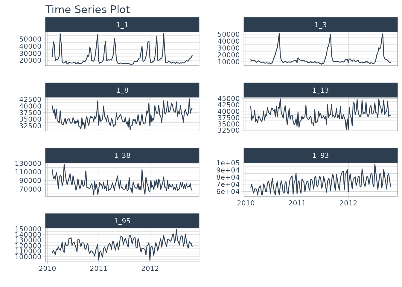
Next, we load the walmart_sales_weekly data containing 7
time series and visualize them using the
timetk::plot_time_series() function.
data_tbl <- walmart_sales_weekly %>%
    select(id, Date, Weekly_Sales)

data_tbl %>%
  group_by(id) %>%
  plot_time_series(
      .date_var    = Date,
      .value       = Weekly_Sales,
      .facet_ncol  = 2,
      .smooth      = F,
      .interactive = F
  )
Then, we separate the data with the time_series_split()
function and generate a training dataset and a test one.
splits <- time_series_split(data_tbl, assess = "3 month", cumulative = TRUE)

recipe_spec <- recipe(Weekly_Sales ~ ., data = training(splits)) %>%
    step_timeseries_signature(Date)

train_tbl <- training(splits) %>% bake(prep(recipe_spec), .)
test_tbl  <- testing(splits) %>% bake(prep(recipe_spec), .)
Model specification, training and prediction
In order to correctly use modeltime.h2o, it is necessary to connect
to an H2O cluster through the h2o.init() function. You can
find more information on how to set up the cluster by typing
?h2o.init or by visiting the official
site.
# Initialize H2O
h2o.init(
    nthreads = -1,
    ip       = 'localhost',
    port     = 54321
)
#>
#> H2O is not running yet, starting it now...
#>
#> Note:  In case of errors look at the following log files:
#>     /tmp/RtmpD7NvJJ/file217c797e529f/h2o_runner_started_from_r.out
#>     /tmp/RtmpD7NvJJ/file217c77a3486f/h2o_runner_started_from_r.err
#>
#>
#> Starting H2O JVM and connecting: .... Connection successful!
#>
#> R is connected to the H2O cluster:
#>     H2O cluster uptime:         1 seconds 919 milliseconds
#>     H2O cluster timezone:       UTC
#>     H2O data parsing timezone:  UTC
#>     H2O cluster version:        3.42.0.2
#>     H2O cluster version age:    5 months and 10 days
#>     H2O cluster name:           H2O_started_from_R_runner_wle394
#>     H2O cluster total nodes:    1
#>     H2O cluster total memory:   3.90 GB
#>     H2O cluster total cores:    4
#>     H2O cluster allowed cores:  4
#>     H2O cluster healthy:        TRUE
#>     H2O Connection ip:          localhost
#>     H2O Connection port:        54321
#>     H2O Connection proxy:       NA
#>     H2O Internal Security:      FALSE
#>     R Version:                  R version 4.3.2 (2023-10-31)

# Optional - Set H2O No Progress to remove progress bars
h2o.no_progress()
Now comes the fun part! We define our model specification with the
automl_reg() function and pass the arguments through the
engine:
model_spec <- automl_reg(mode = 'regression') %>%
    set_engine(
         engine                     = 'h2o',
         max_runtime_secs           = 5,
         max_runtime_secs_per_model = 3,
         max_models                 = 3,
         nfolds                     = 5,
         exclude_algos              = c("DeepLearning"),
         verbosity                  = NULL,
         seed                       = 786
    )

model_spec
#> H2O AutoML Model Specification (regression)
#>
#> Engine-Specific Arguments:
#>   max_runtime_secs = 5
#>   max_runtime_secs_per_model = 3
#>   max_models = 3
#>   nfolds = 5
#>   exclude_algos = c("DeepLearning")
#>   verbosity = NULL
#>   seed = 786
#>
#> Computational engine: h2o
Next, let’s train the model with fit()!
model_fitted <- model_spec %>%
    fit(Weekly_Sales ~ ., data = train_tbl)
#>                                                  model_id      rmse        mse
#> 1                      XGBoost_1_AutoML_1_20240104_204414  6368.842   40562143
#> 2 StackedEnsemble_BestOfFamily_1_AutoML_1_20240104_204414  6371.445   40595317
#> 3                          GBM_1_AutoML_1_20240104_204414  7607.165   57868955
#> 4                          GLM_1_AutoML_1_20240104_204414 36255.636 1314471115
#>         mae     rmsle mean_residual_deviance
#> 1  4175.752 0.1753395               40562143
#> 2  4107.600 0.1690209               40595317
#> 3  5125.090 0.2115567               57868955
#> 4 31032.413 0.8352711             1314471115
#>
#> [4 rows x 6 columns]

model_fitted
#> parsnip model object
#>
#>
#> H2O AutoML - Xgboost
#> --------
#> Model: Model Details:
#> ==============
#>
#> H2ORegressionModel: xgboost
#> Model ID:  XGBoost_1_AutoML_1_20240104_204414
#> Model Summary:
#>   number_of_trees
#> 1              44
#>
#>
#> H2ORegressionMetrics: xgboost
#> ** Reported on training data. **
#>
#> MSE:  8905205
#> RMSE:  2984.159
#> MAE:  2011.225
#> RMSLE:  0.09321704
#> Mean Residual Deviance :  8905205
#>
#>
#>
#> H2ORegressionMetrics: xgboost
#> ** Reported on cross-validation data. **
#> ** 5-fold cross-validation on training data (Metrics computed for combined holdout predictions) **
#>
#> MSE:  40562143
#> RMSE:  6368.842
#> MAE:  4175.752
#> RMSLE:  0.1753395
#> Mean Residual Deviance :  40562143
#>
#>
#> Cross-Validation Metrics Summary:
#>                                   mean              sd      cv_1_valid
#> mae                        4175.762000      272.333200     3890.696000
#> mean_residual_deviance 40559876.000000 11151054.000000 28802630.000000
#> mse                    40559876.000000 11151054.000000 28802630.000000
#> r2                            0.969156        0.008390        0.977998
#> residual_deviance      40559876.000000 11151054.000000 28802630.000000
#> rmse                       6320.693400      872.290200     5366.808000
#> rmsle                         0.174745        0.016217        0.153008
#>                             cv_2_valid      cv_3_valid      cv_4_valid
#> mae                        4450.958500     4100.722700     4473.589400
#> mean_residual_deviance 54395072.000000 37792108.000000 49844588.000000
#> mse                    54395072.000000 37792108.000000 49844588.000000
#> r2                            0.958720        0.971498        0.962121
#> residual_deviance      54395072.000000 37792108.000000 49844588.000000
#> rmse                       7375.302000     6147.529000     7060.070000
#> rmsle                         0.189853        0.171167        0.191813
#>                             cv_5_valid
#> mae                        3962.845000
#> mean_residual_deviance 31964988.000000
#> mse                    31964988.000000
#> r2                            0.975442
#> residual_deviance      31964988.000000
#> rmse                       5653.759000
#> rmsle                         0.167883
The best models are stored in the leaderbord and by
default the one with the best metric with which you have decided to sort
the leaderbord is selected (this behavior can be controlled with the
sort_metric parameter passed through set_engine. For more
information see ?h2o.automl. By default, it is sorted by the
mean_residual_deviance). To list the models created during training that
have finally been stored in the leaderbord you can use the
automl_leaderbord function as follows:
automl_leaderboard(model_fitted)
#> # A tibble: 4 × 6
#>   model_id                       rmse    mse    mae rmsle mean_residual_deviance
#>   <chr>                         <dbl>  <dbl>  <dbl> <dbl>                  <dbl>
#> 1 XGBoost_1_AutoML_1_20240104…  6369. 4.06e7  4176. 0.175              40562143.
#> 2 StackedEnsemble_BestOfFamil…  6371. 4.06e7  4108. 0.169              40595317.
#> 3 GBM_1_AutoML_1_20240104_204…  7607. 5.79e7  5125. 0.212              57868955.
#> 4 GLM_1_AutoML_1_20240104_204… 36256. 1.31e9 31032. 0.835            1314471115.
To change the default selected model (remember, the first one sorted
according to the selected metric) you can do it with the
automl_update_model() function as follows (do not run the
following example as the model id name will have changed as there is
randomness in the process):
automl_update_model(model_fitted, model_id = "StackedEnsemble_AllModels_AutoML_20210319_204825")Finally, we predict() on the test dataset:
predict(model_fitted, test_tbl)
#> # A tibble: 84 × 1
#>      .pred
#>      <dbl>
#>  1  19484.
#>  2  33369.
#>  3  37997.
#>  4  40721.
#>  5  70083.
#>  6  81469.
#>  7 136557.
#>  8  14242.
#>  9  34078.
#> 10  35966.
#> # ℹ 74 more rows
Modeltime Workflow
Once we have our fitted model, we can follow the Modeltime Workflow:
Add fitted models to a Model Table.
Calibrate the models to a testing set.
Perform Testing Set Forecast Evaluation & Accuracy Evaluation.
Refit the models to Full Dataset & Forecast Forward
Add fitted models to a Model Table
First, we create the model table:
modeltime_tbl <- modeltime_table(
model_fitted
)
modeltime_tbl
#> # Modeltime Table
#> # A tibble: 1 × 3
#> .model_id .model .model_desc
#> <int> <list> <chr>
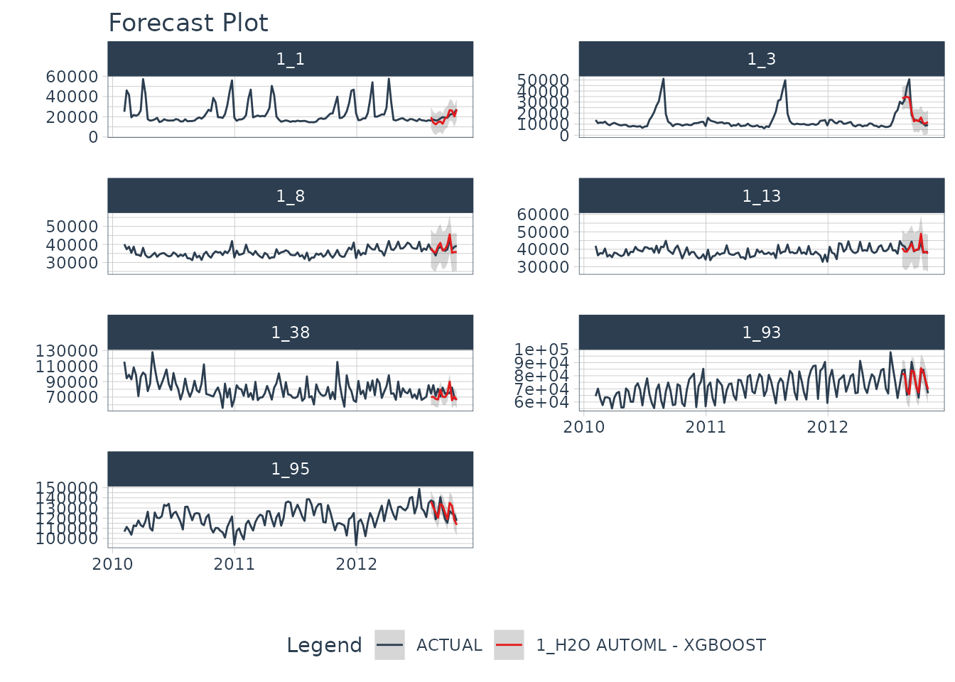
#> 1 1 <fit[+]> H2O AUTOML - XGBOOSTCalibrate & Testing Set Forecast & Accuracy Evaluation
Next, we calibrate to the testing set and visualize the forecasts:
modeltime_tbl %>%
  modeltime_calibrate(test_tbl) %>%
    modeltime_forecast(
        new_data    = test_tbl,
        actual_data = data_tbl,
        keep_data   = TRUE
    ) %>%
    group_by(id) %>%
    plot_modeltime_forecast(
        .facet_ncol = 2,
        .interactive = FALSE
    )
Refit to Full Dataset & Forecast Forward
Before using refit on our dataset, let’s prepare our
data. We create data_prepared_tbl which represents the
complete dataset (the union of train and test) with the variables
created with the recipe named recipe_spec. Subsequently, we create the
dataset future_prepared_tbl that represents the dataset
with the future data to one year and the required variables.
data_prepared_tbl <- bind_rows(train_tbl, test_tbl)

future_tbl <- data_prepared_tbl %>%
    group_by(id) %>%
    future_frame(.length_out = "1 year") %>%
    ungroup()

future_prepared_tbl <- bake(prep(recipe_spec), future_tbl)
Finally, we use forecast in our future dataset and visualize the results once we had reffited.
refit_tbl <- modeltime_tbl %>%
    modeltime_refit(data_prepared_tbl)
#>                                                  model_id      rmse        mse
#> 1                      XGBoost_1_AutoML_2_20240104_204427  6060.518   36729882
#> 2 StackedEnsemble_BestOfFamily_1_AutoML_2_20240104_204427  6061.512   36741927
#> 3                          GBM_1_AutoML_2_20240104_204427  7524.808   56622738
#> 4                          GLM_1_AutoML_2_20240104_204427 36259.518 1314752625
#>         mae     rmsle mean_residual_deviance
#> 1  4075.988 0.1677377               36729882
#> 2  3998.426 0.1604279               36741927
#> 3  5163.899 0.2088567               56622738
#> 4 31017.107 0.8289850             1314752625
#>
#> [4 rows x 6 columns]

refit_tbl %>%
    modeltime_forecast(
        new_data    = future_prepared_tbl,
        actual_data = data_prepared_tbl,
        keep_data   = TRUE
    ) %>%
    group_by(id) %>%
    plot_modeltime_forecast(
        .facet_ncol  = 2,
        .interactive = FALSE
    )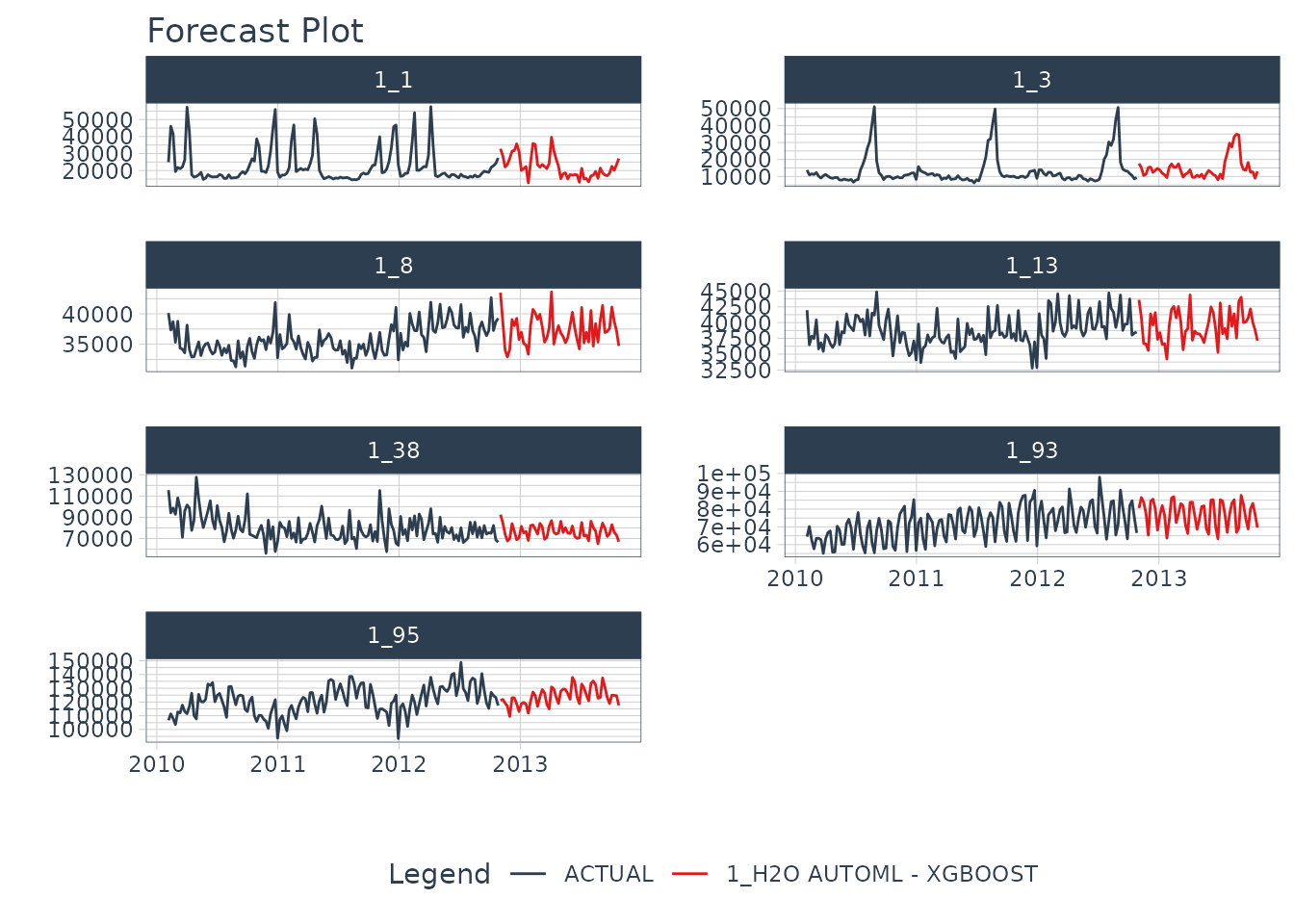
We can likely do better than this if we train longer but really good for a quick example!
Saving and Loading Models
H2O models will need to “serialized” (a fancy word for saved to a
directory that contains the recipe for recreating the models). To save
the models, use save_h2o_model().
- Provide a directory where you want to save the model.
- This saves the model file in the directory.
model_fitted %>%
  save_h2o_model(path = "../model_fitted", overwrite = TRUE)
You can reload the model into R using
load_h2o_model().
model_h2o <- load_h2o_model(path = "../model_fitted/")Shut down H2O when finished
Finally, once we have saved the specific models that we want to keep, we shutdown the H2O cluster.
h2o.shutdown(prompt = FALSE)Need to learn high-performance time series forecasting?
Take the High-Performance Forecasting Course
Become the forecasting expert for your organization
High-Performance Time Series Course
Time Series is Changing
Time series is changing. Businesses now need 10,000+ time series forecasts every day. This is what I call a High-Performance Time Series Forecasting System (HPTSF) - Accurate, Robust, and Scalable Forecasting.
High-Performance Forecasting Systems will save companies by improving accuracy and scalability. Imagine what will happen to your career if you can provide your organization a “High-Performance Time Series Forecasting System” (HPTSF System).
How to Learn High-Performance Time Series Forecasting
I teach how to build a HPTFS System in my High-Performance Time Series Forecasting Course. You will learn:
-
Time Series Machine Learning (cutting-edge) with
Modeltime- 30+ Models (Prophet, ARIMA, XGBoost, Random Forest, & many more) -
Deep Learning with
GluonTS(Competition Winners) - Time Series Preprocessing, Noise Reduction, & Anomaly Detection
- Feature engineering using lagged variables & external regressors
- Hyperparameter Tuning
- Time series cross-validation
- Ensembling Multiple Machine Learning & Univariate Modeling Techniques (Competition Winner)
- Scalable Forecasting - Forecast 1000+ time series in parallel
- and more.
Become the Time Series Expert for your organization.