Getting Started with Modeltime GluonTS

Making an DeepAR Model

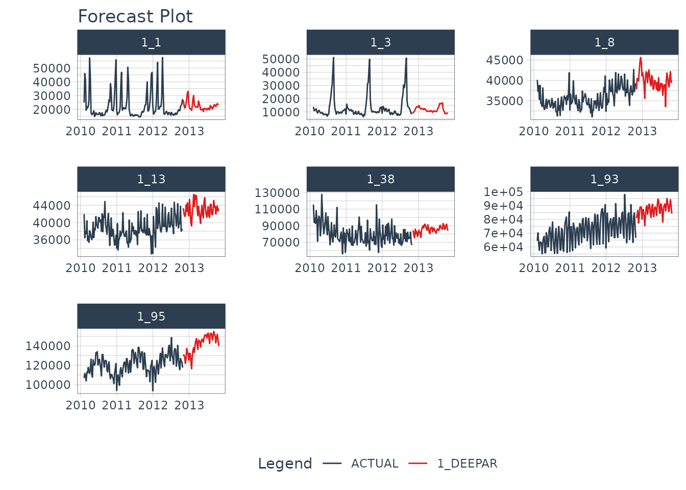
Let’s get started by making a DeepAR Model. In a matter of minutes, you’ll generate the 7 forecasts shown below. If you’d like to improve your time series forecasting abilities, then please take my High-Performance Time Series Course.

Libraries

Load the following libraries.

library(modeltime.gluonts)
library(tidymodels)
library(tidyverse)
library(timetk)

Installation

Next, set up the Python Environment with install_gluonts(). You only need to run this one time, and then you are good to go.

install_gluonts()

We have a more detailed installation instructions and troubleshooting guidance in our Installation Guide.

Time Series Data

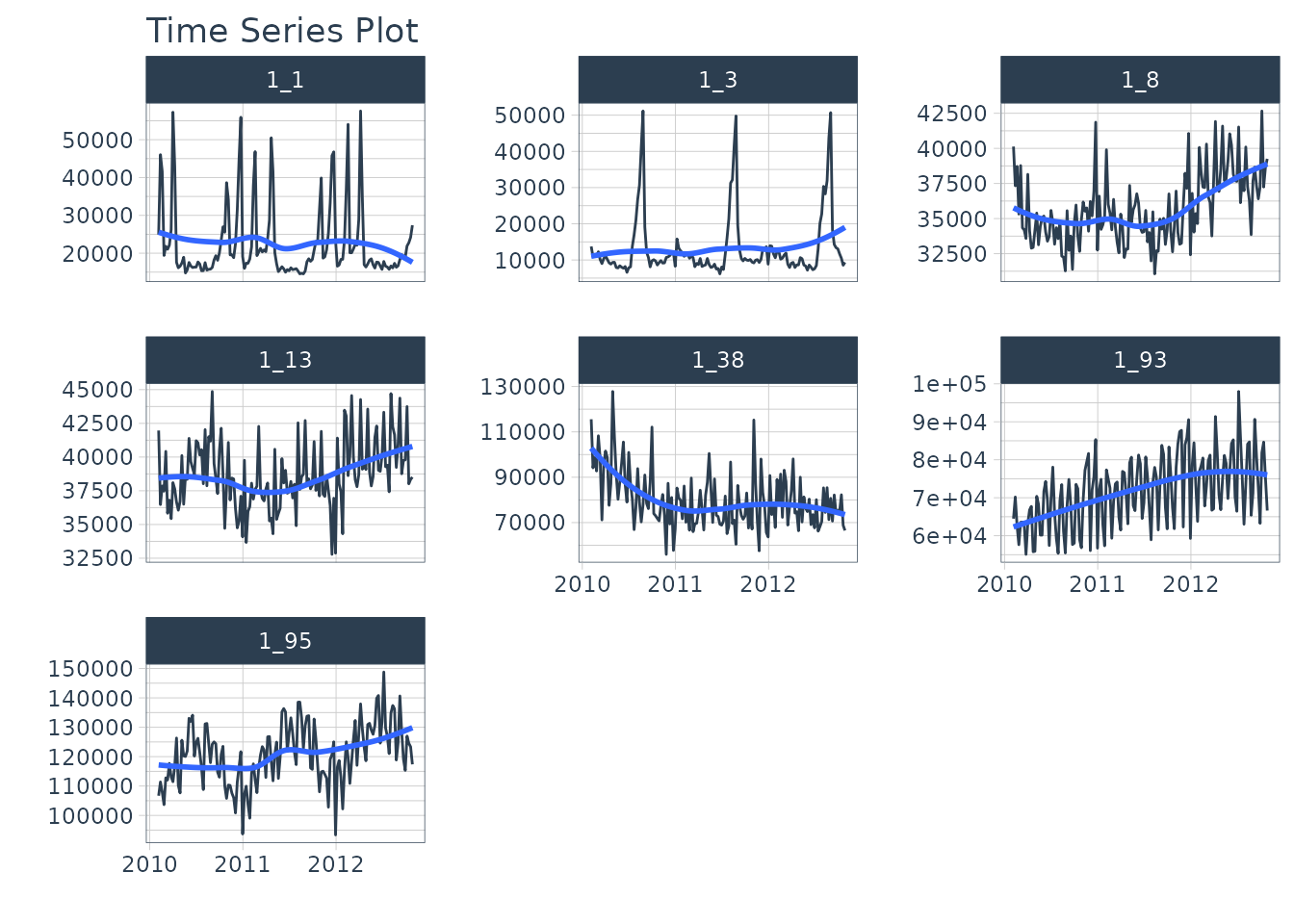
We’ll use the walmart_sales_weekly dataset, which contains 7 weekly time series of sales data for various departments in a Walmart Store.

data <- walmart_sales_weekly %>%
  select(id, Date, Weekly_Sales) %>%
  set_names(c("id", "date", "value"))

data %>%
  group_by(id) %>%
  plot_time_series(
    date, 
    value, 
    .facet_ncol = 3, 
    .interactive = FALSE
  )

We’ll create the forecast region using future_frame(). We are forecasting 1 week (24x7 timestamps) into the future.

HORIZON <- 52

new_data <- data %>%
  group_by(id) %>%
  future_frame(.length_out = HORIZON) %>%
  ungroup()

new_data
#> # A tibble: 364 × 2
#>    id    date      
#>    <fct> <date>    
#>  1 1_1   2012-11-02
#>  2 1_1   2012-11-09
#>  3 1_1   2012-11-16
#>  4 1_1   2012-11-23
#>  5 1_1   2012-11-30
#>  6 1_1   2012-12-07
#>  7 1_1   2012-12-14
#>  8 1_1   2012-12-21
#>  9 1_1   2012-12-28
#> 10 1_1   2013-01-04
#> # ℹ 354 more rows

Making a DeepAR Model

We’ll create a DeepAR model using the deep_ar() function.

• This is a univariate modeling algorithm that uses Deep Learning and Autoregression.
• We select the GluonTS version by setting the engine to gluonts_deepar.

model_fit_deepar <- deep_ar(
  id                    = "id",
  freq                  = "W",
  prediction_length     = HORIZON,
  lookback_length       = 2*HORIZON,
  epochs                = 5
) %>%
  set_engine("gluonts_deepar") %>%
  fit(value ~ date + id, data)

Forecasting

With a model in hand, we can simply follow the Modeltime Workflow to generate a forecast for the multiple time series groups.

modeltime_forecast_tbl <- modeltime_table(
  model_fit_deepar
) %>%
  modeltime_forecast(
    new_data    = new_data,
    actual_data = data,
    keep_data   = TRUE
  ) %>%
  group_by(id) 

We can visualize the forecast with plot_modeltime_forecast().

modeltime_forecast_tbl %>%
  plot_modeltime_forecast(
    .conf_interval_show = FALSE, 
    .facet_ncol         = 3, 
    .facet_scales       = "free",
    .interactive        = FALSE
  )

Saving and Loading Models

GluonTS models will need to “serialized” (a fancy word for saved to a directory that contains the recipe for recreating the models). To save the models, use save_gluonts_model().

• Provide a directory where you want to save the model.
• This saves all of the model files in the directory.

model_fit_deepar %>%
  save_gluonts_model(path = "deepar_model", overwrite = TRUE)

You can reload the model into R using load_gluonts_model().

model_fit_deepar <- load_gluonts_model("deepar_model")

Take the High-Performance Forecasting Course

Become the forecasting expert for your organization

High-Performance Time Series Course

Time Series is Changing

Time series is changing. Businesses now need 10,000+ time series forecasts every day. This is what I call a High-Performance Time Series Forecasting System (HPTSF) - Accurate, Robust, and Scalable Forecasting.

High-Performance Forecasting Systems will save companies by improving accuracy and scalability. Imagine what will happen to your career if you can provide your organization a “High-Performance Time Series Forecasting System” (HPTSF System).

How to Learn High-Performance Time Series Forecasting

I teach how to build a HPTFS System in my High-Performance Time Series Forecasting Course. You will learn:

• Time Series Machine Learning (cutting-edge) with Modeltime - 30+ Models (Prophet, ARIMA, XGBoost, Random Forest, & many more)
• Deep Learning with GluonTS (Competition Winners)
• Time Series Preprocessing, Noise Reduction, & Anomaly Detection
• Feature engineering using lagged variables & external regressors
• Hyperparameter Tuning
• Time series cross-validation
• Ensembling Multiple Machine Learning & Univariate Modeling Techniques (Competition Winner)
• Scalable Forecasting - Forecast 1000+ time series in parallel
• and more.

Become the Time Series Expert for your organization.

Take the High-Performance Time Series Forecasting Course