Getting Started with Modeltime Resample

Modeltime Resample provide a convenient toolkit for efficiently evaluating multiple models across time, increasing our confidence in model selections.

• The core functionality is modeltime_resample(), which automates the iterative model fitting and prediction procedure.
• A new plotting function plot_modeltime_resamples() provides a quick way to review model resample accuracy visually.
• A new accuracy function modeltime_resample_accuracy() provides a flexible way for creating custom accuracy tables using customizable summary functions (e.g. mean, median, sd, min, max).

Single Time Series

Resampling gives us a way to compare multiple models across time.

In this tutorial, we’ll get you up to speed by evaluating multiple models using resampling of a single time series.

Getting Started Setup

Load the following R packages.

library(tidymodels)
library(modeltime)
library(modeltime.resample)
library(tidyverse)
library(timetk)

We’ll work with the m750 data set.

m750 %>%
  plot_time_series(date, value, .interactive = FALSE)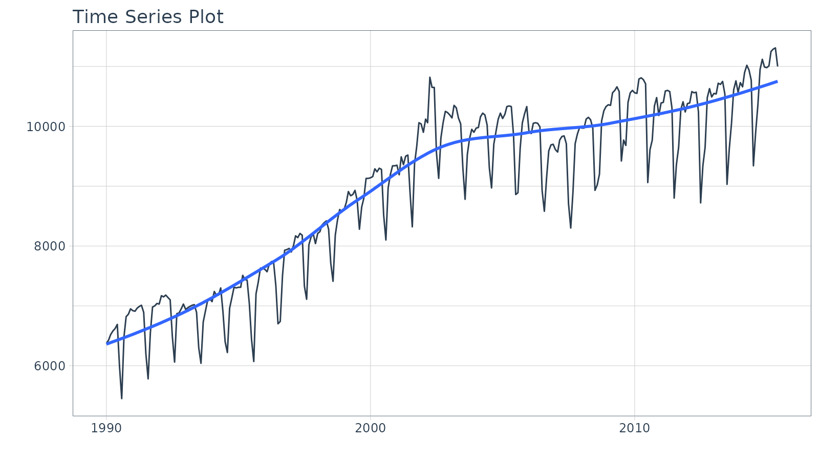

Step 1 - Make a Cross-Validation Training Plan

We’ll use timetk::time_series_cv() to generate 4 time-series resamples.

• Assess is the assessment window: "2 years"
• Initial is the training window: "5 years"
• Skip is the shift between resample sets: "2 years
• Slice Limit is how many resamples to generate: 4

resamples_tscv <- time_series_cv(
    data        = m750,
    assess      = "2 years",
    initial     = "5 years",
    skip        = "2 years",
    slice_limit = 4
)

resamples_tscv

## # Time Series Cross Validation Plan 
## # A tibble: 4 × 2
##   splits          id    
##   <list>          <chr> 
## 1 <split [60/24]> Slice1
## 2 <split [60/24]> Slice2
## 3 <split [60/24]> Slice3
## 4 <split [60/24]> Slice4

Next, visualize the resample strategy to make sure we’re happy with our choices.

# Begin with a Cross Validation Strategy
resamples_tscv %>%
    tk_time_series_cv_plan() %>%
    plot_time_series_cv_plan(date, value, .facet_ncol = 2, .interactive = FALSE)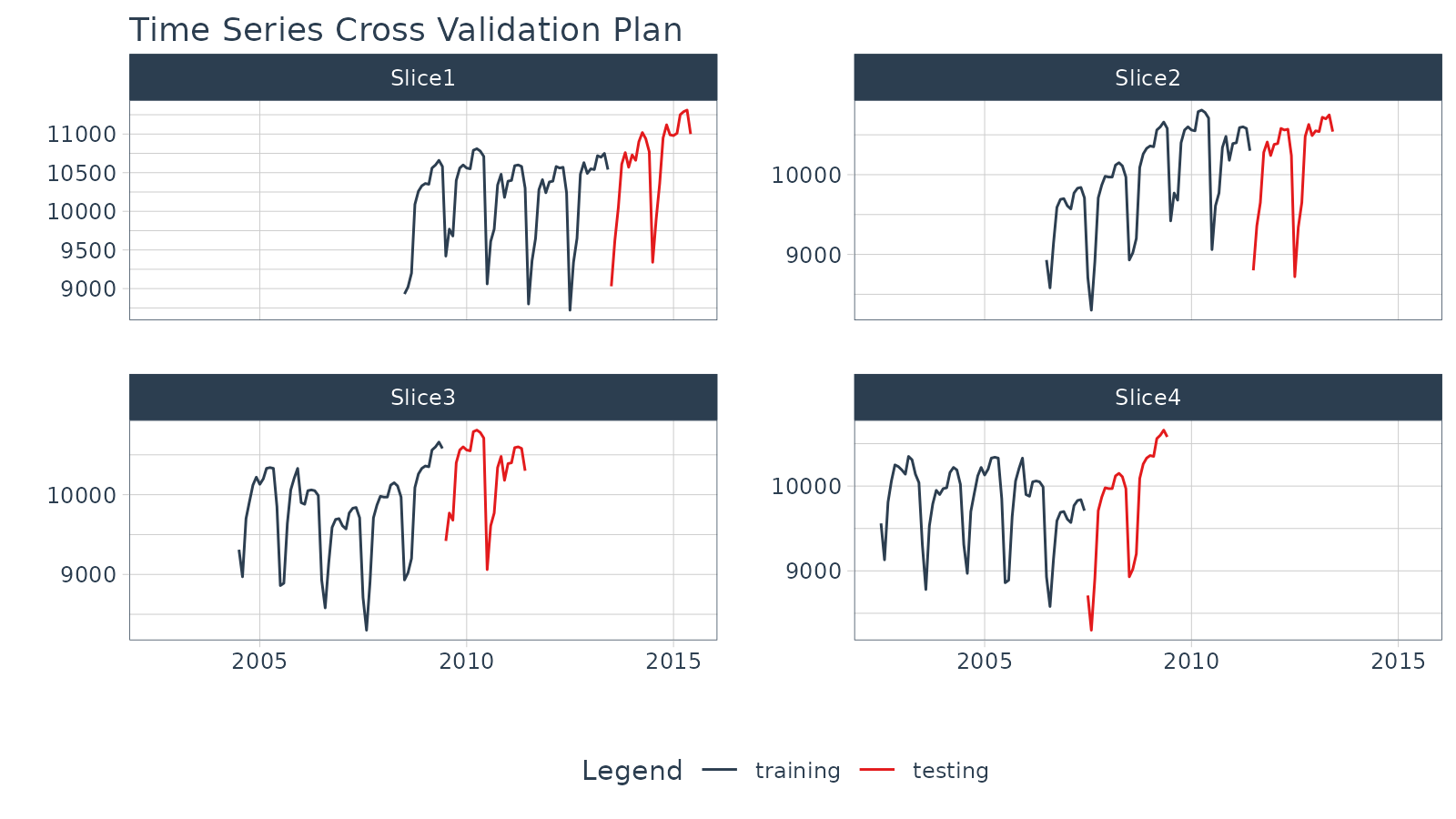

Step 2 - Make a Modeltime Table

Create models and add them to a Modeltime Table with Modeltime. I’ve already created 3 models (ARIMA, Prophet, and GLMNET) and saved the results as part of the modeltime package m750_models.

m750_models

## # Modeltime Table
## # A tibble: 3 × 3
##   .model_id .model     .model_desc            
##       <int> <list>     <chr>                  
## 1         1 <workflow> ARIMA(0,1,1)(0,1,1)[12]
## 2         2 <workflow> PROPHET                
## 3         3 <workflow> GLMNET

Step 3 - Generate Resample Predictions

Generate resample predictions using modeltime_fit_resamples():

• Use the m750_models (models) and m750_training_resamples
• Internally, each model is refit to each training set of the resamples
• A column is added to the Modeltime Table: .resample_results contains the resample predictions

resamples_fitted <- m750_models %>%
    modeltime_fit_resamples(
        resamples = resamples_tscv,
        control   = control_resamples(verbose = FALSE)
    )

resamples_fitted

## # Modeltime Table
## # A tibble: 3 × 4
##   .model_id .model     .model_desc             .resample_results
##       <int> <list>     <chr>                   <list>           
## 1         1 <workflow> ARIMA(0,1,1)(0,1,1)[12] <tibble [4 × 4]> 
## 2         2 <workflow> PROPHET                 <tibble [4 × 4]> 
## 3         3 <workflow> GLMNET                  <tibble [4 × 4]>

Step 4 - Evaluate the Results

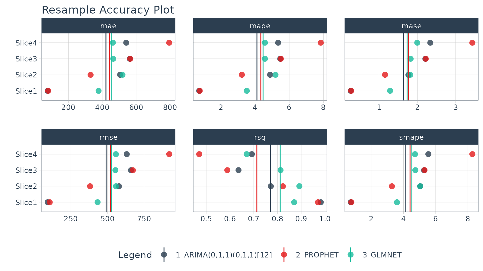
Accuracy Plot

Visualize the model resample accuracy using plot_modeltime_resamples(). Some observations:

• Overall: The ARIMA has the best overall performance, but it’s not always the best.
• Slice 4: We can see that Slice 4 seems to be giving the models the most issue. The GLMNET model is relatively robust to Slice 4. Prophet gets thrown for a loop.

resamples_fitted %>%
    plot_modeltime_resamples(
      .point_size  = 3, 
      .point_alpha = 0.8,
      .interactive = FALSE
    )

Accuracy Table

We can compare the overall modeling approaches by evaluating the results with modeltime_resample_accuracy(). The default is to report the average summary_fns = mean, but this can be changed to any summary function or a list containing multiple summary functions (e.g. summary_fns = list(mean = mean, sd = sd)). From the table below, ARIMA has a 6% lower RMSE, indicating it’s the best choice for consistent performance on this dataset.

resamples_fitted %>%
    modeltime_resample_accuracy(summary_fns = mean) %>%
    table_modeltime_accuracy(.interactive = FALSE)

Accuracy Table
.model_id	.model_desc	.type	n	mae	mape	mase	smape	rmse	rsq
1	ARIMA(0,1,1)(0,1,1)[12]	Resamples	4	421.78	4.11	1.64	4.15	490.88	0.77
2	PROPHET	Resamples	4	443.09	4.34	1.77	4.41	520.80	0.71
3	GLMNET	Resamples	4	456.33	4.47	1.73	4.52	525.89	0.81

Wrapup

Resampling gives us a way to compare multiple models across time. In this example, we can see that the ARIMA model performs better than the Prophet and GLMNET models with a lower RMSE. This won’t always be the case (every time series is different).

This is a quick overview of Getting Started with Modeltime Resample. To learn how to tune, ensemble, and work with multiple groups of Time Series, take my High-Performance Time Series Course.