Reduce Forecast Error with Cleaned Anomalies
Business Science
2023-12-28
Source:vignettes/forecasting_with_cleaned_anomalies.Rmd
forecasting_with_cleaned_anomalies.RmdForecasting error can often be reduced 20% to 50% by repairing anomolous data
Example - Reducing Forecasting Error by 32%
We can often get better forecast performance by cleaning anomalous
data prior to forecasting. This is the perfect use case for integrating
the clean_anomalies() function into your
forecast workflow.
# NOTE: timetk now has anomaly detection built in, which
#  will get the new functionality going forward.
#  Use this script to prevent overwriting legacy anomalize:

anomalize <- anomalize::anomalize
plot_anomalies <- anomalize::plot_anomalies
Here is a short example with the
tidyverse_cran_downloads dataset that comes with
anomalize. We’ll see how we can reduce the forecast
error by 32% simply by repairing anomalies.
tidyverse_cran_downloads
#> # A tibble: 6,375 × 3
#> # Groups:   package [15]
#>    date       count package
#>    <date>     <dbl> <chr>
#>  1 2017-01-01   873 tidyr
#>  2 2017-01-02  1840 tidyr
#>  3 2017-01-03  2495 tidyr
#>  4 2017-01-04  2906 tidyr
#>  5 2017-01-05  2847 tidyr
#>  6 2017-01-06  2756 tidyr
#>  7 2017-01-07  1439 tidyr
#>  8 2017-01-08  1556 tidyr
#>  9 2017-01-09  3678 tidyr
#> 10 2017-01-10  7086 tidyr
#> # ℹ 6,365 more rows
Let’s take one package with some extreme events. We can hone in on
lubridate, which has some outliers that we can fix.
tidyverse_cran_downloads %>%
  ggplot(aes(date, count, color = package)) +
  geom_point(alpha = 0.5) +
  facet_wrap(~ package, ncol = 3, scales = "free_y") +
  scale_color_viridis_d() +
theme_tq() 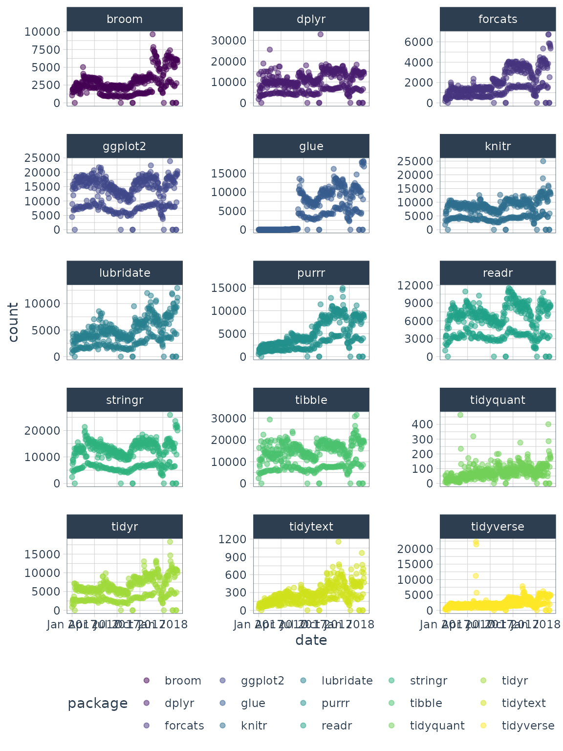
Forecasting Lubridate Downloads
Let’s focus on downloads of the lubridate R package.
First, we’ll make a function, forecast_mae(), that can
take the input of both cleaned and uncleaned anomalies and calculate
forecast error of future uncleaned anomalies.
The modeling function uses the following criteria:
- Split the
datainto training and testing data that maintains the correct time-series sequence using thepropargument. - Models the daily time series of the training data set from observed
(demonstrates no cleaning) or observed and cleaned (demonstrates
improvement from cleaning). Specified by the
col_trainargument. - Compares the predictions to the observed values. Specified by the
col_testargument.
forecast_mae <- function(data, col_train, col_test, prop = 0.8) {

  predict_expr <- enquo(col_train)
  actual_expr <- enquo(col_test)

  idx_train <- 1:(floor(prop * nrow(data)))

  train_tbl <- data %>% filter(row_number() %in% idx_train)
  test_tbl  <- data %>% filter(!row_number() %in% idx_train)

  # Model using training data (training)
  model_formula <- as.formula(paste0(quo_name(predict_expr), " ~ index.num + year + quarter + month.lbl + day + wday.lbl"))

  model_glm <- train_tbl %>%
    tk_augment_timeseries_signature() %>%
    glm(model_formula, data = .)

  # Make Prediction
  suppressWarnings({
    # Suppress rank-deficit warning
    prediction <- predict(model_glm, newdata = test_tbl %>% tk_augment_timeseries_signature())
    actual     <- test_tbl %>% pull(!! actual_expr)
  })

  # Calculate MAE
  mae <- mean(abs(prediction - actual))

  return(mae)

}
Workflow for Cleaning Anomalies
We will use the anomalize workflow of decomposing
(time_decompose()) and identifying anomalies
(anomalize()). We use the function,
clean_anomalies(), to add new column called
“observed_cleaned” that is repaired by replacing all anomalies with the
trend + seasonal components from the decompose operation. We
can now experiment to see the improvment in forecasting performance by
comparing a forecast made with “observed” versus “observed_cleaned”
lubridate_anomalized_tbl <- lubridate_tbl %>%
  time_decompose(count) %>%
  anomalize(remainder) %>%

  # Function to clean & repair anomalous data
  clean_anomalies()
#> Converting from tbl_df to tbl_time.
#> Auto-index message: index = date
#> frequency = 7 days
#> trend = 91 days

lubridate_anomalized_tbl
#> # A time tibble: 425 × 9
#> # Index:         date
#>    date       observed season trend remainder remainder_l1 remainder_l2 anomaly
#>    <date>        <dbl>  <dbl> <dbl>     <dbl>        <dbl>        <dbl> <chr>
#>  1 2017-01-01      643 -2078. 2474.      246.       -3323.        3310. No
#>  2 2017-01-02     1350   518. 2491.    -1659.       -3323.        3310. No
#>  3 2017-01-03     2940  1117. 2508.     -685.       -3323.        3310. No
#>  4 2017-01-04     4269  1220. 2524.      525.       -3323.        3310. No
#>  5 2017-01-05     3724   865. 2541.      318.       -3323.        3310. No
#>  6 2017-01-06     2326   356. 2558.     -588.       -3323.        3310. No
#>  7 2017-01-07     1107 -1998. 2574.      531.       -3323.        3310. No
#>  8 2017-01-08     1058 -2078. 2591.      545.       -3323.        3310. No
#>  9 2017-01-09     2494   518. 2608.     -632.       -3323.        3310. No
#> 10 2017-01-10     3237  1117. 2624.     -504.       -3323.        3310. No
#> # ℹ 415 more rows
#> # ℹ 1 more variable: observed_cleaned <dbl>
Before Cleaning with anomalize
lubridate_anomalized_tbl %>%
  forecast_mae(col_train = observed, col_test = observed, prop = 0.8)
#> tk_augment_timeseries_signature(): Using the following .date_var variable: date
#> tk_augment_timeseries_signature(): Using the following .date_var variable: date
#> [1] 4054.053
After Cleaning with anomalize
lubridate_anomalized_tbl %>%
  forecast_mae(col_train = observed_cleaned, col_test = observed, prop = 0.8)
#> tk_augment_timeseries_signature(): Using the following .date_var variable: date
#> tk_augment_timeseries_signature(): Using the following .date_var variable: date
#> [1] 2755.297
32% Reduction in Forecast Error
This is approximately a 32% reduction in forecast error as measure by Mean Absolute Error (MAE).
(2755 - 4054) / 4054
#> [1] -0.3204243
Interested in Learning Anomaly Detection?
Business Science offers two 1-hour courses on Anomaly Detection:
Learning Lab 18 - Time Series Anomaly Detection with
anomalizeLearning Lab 17 - Anomaly Detection with
H2OMachine Learning