Introduction to sweep

Extending broom to time series forecasting

The sweep package extends the broom tools (tidy, glance, and augment) for performing forecasts and time series analysis in the “tidyverse”. The package is geared towards the workflow required to perform forecasts using Rob Hyndman’s forecast package, and contains the following elements:

model tidiers: sw_tidy, sw_glance, sw_augment, sw_tidy_decomp functions extend tidy, glance, and augment from the broom package specifically for models (ets(), Arima(), bats(), etc) used for forecasting.
forecast tidier: sw_sweep converts a forecast object to a tibble that can be easily manipulated in the “tidyverse”.

To illustrate, let’s take a basic forecasting workflow starting from data collected in a tibble format and then performing a forecast to achieve the end result in tibble format.

Prerequisites

Before we get started, load the following packages.

library(ggplot2)
library(tidyquant)
library(timetk)
library(sweep)
library(forecast)

Forecasting Sales of Beer, Wine, and Distilled Alcohol Beverages

We’ll use the tidyquant package to get the US alcohol sales, which comes from the FRED data base (the origin is the US Bureau of the Census, one of the 80+ data sources FRED connects to). The FRED code is “S4248SM144NCEN” and the data set can be found here.

alcohol_sales_tbl <- tq_get("S4248SM144NCEN", 
                            get  = "economic.data", 
                            from = "2007-01-01",
                            to   = "2016-12-31")
alcohol_sales_tbl

## # A tibble: 120 × 3
##    symbol         date       price
##    <chr>          <date>     <int>
##  1 S4248SM144NCEN 2007-01-01  6627
##  2 S4248SM144NCEN 2007-02-01  6743
##  3 S4248SM144NCEN 2007-03-01  8195
##  4 S4248SM144NCEN 2007-04-01  7828
##  5 S4248SM144NCEN 2007-05-01  9570
##  6 S4248SM144NCEN 2007-06-01  9484
##  7 S4248SM144NCEN 2007-07-01  8608
##  8 S4248SM144NCEN 2007-08-01  9543
##  9 S4248SM144NCEN 2007-09-01  8123
## 10 S4248SM144NCEN 2007-10-01  9649
## # ℹ 110 more rows

We can quickly visualize using the ggplot2 package. We can see that there appears to be some seasonality and an upward trend.

alcohol_sales_tbl %>%
    ggplot(aes(x = date, y = price)) +
    geom_line(linewidth = 1, color = palette_light()[[1]]) +
    geom_smooth(method = "loess") +
    labs(title = "US Alcohol Sales: Monthly", x = "", y = "Millions") +
    scale_y_continuous(labels = scales::dollar) +
    scale_x_date(date_breaks = "1 year", date_labels = "%Y") +
    theme_tq()

## `geom_smooth()` using formula = 'y ~ x'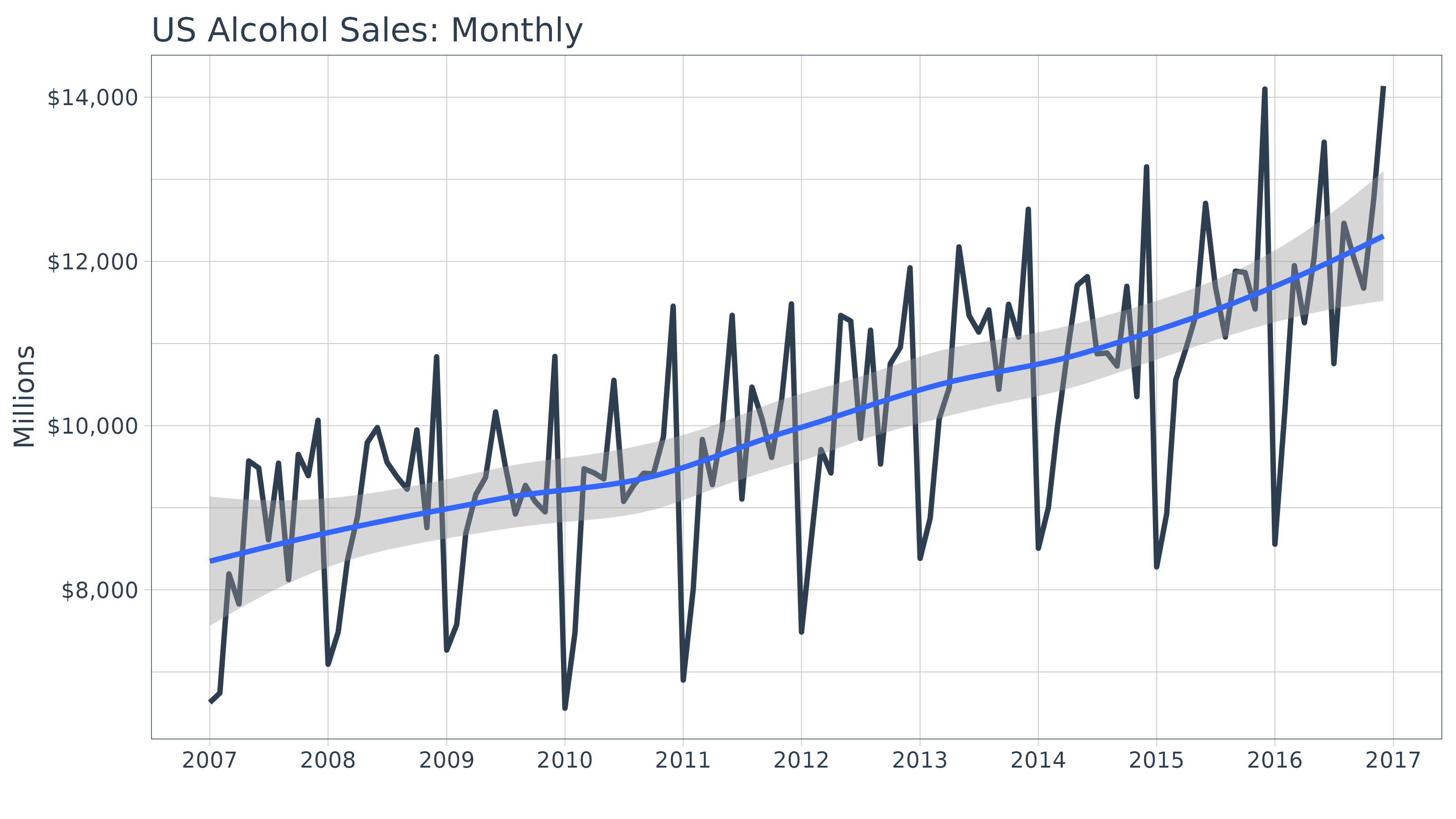

Forecasting Workflow

The forecasting workflow involves a few basic steps:

Step 1: Coerce to a ts object class.
Step 2: Apply a model (or set of models)
Step 3: Forecast the models (similar to predict)
Step 4: Use sw_sweep() to tidy the forecast.

Note that we purposely omit other steps such as testing the series for stationarity (Box.test(type = "Ljung")) and analysis of autocorrelations (Acf, Pacf) for brevity purposes. We recommend the analyst to follow the forecasting workflow in “Forecasting: principles and practice”

Step 1: Coerce to a `ts` object class

The forecast package uses the ts data structure, which is quite a bit different than tibbles that we are currently using. Fortunately, it’s easy to get to the correct structure with tk_ts() from the timetk package. The start and freq variables are required for the regularized time series (ts) class, and these specify how to treat the time series. For monthly, the frequency should be specified as 12. This results in a nice calendar view. The silent = TRUE tells the tk_ts() function to skip the warning notifying us that the “date” column is being dropped. Non-numeric columns must be dropped for ts class, which is matrix based and a homogeneous data class.

alcohol_sales_ts <- tk_ts(alcohol_sales_tbl, start = 2007, freq = 12, silent = TRUE)
alcohol_sales_ts

##        Jan   Feb   Mar   Apr   May   Jun   Jul   Aug   Sep   Oct   Nov   Dec
## 2007  6627  6743  8195  7828  9570  9484  8608  9543  8123  9649  9390 10065
## 2008  7093  7483  8365  8895  9794  9977  9553  9375  9225  9948  8758 10839
## 2009  7266  7578  8688  9162  9369 10167  9507  8923  9272  9075  8949 10843
## 2010  6558  7481  9475  9424  9351 10552  9077  9273  9420  9413  9866 11455
## 2011  6901  8014  9832  9281  9967 11344  9106 10469 10085  9612 10328 11483
## 2012  7486  8641  9709  9423 11342 11274  9845 11163  9532 10754 10953 11922
## 2013  8383  8870 10085 10462 12177 11342 11139 11409 10442 11479 11077 12636
## 2014  8506  9003  9991 10903 11709 11815 10875 10884 10725 11697 10353 13153
## 2015  8279  8926 10557 10933 11330 12708 11700 11079 11882 11865 11420 14100
## 2016  8556 10199 11949 11253 12046 13453 10755 12465 12038 11674 12761 14137

A significant benefit is that the resulting ts object maintains a “timetk index”, which will help with forecasting dates later. We can verify this using has_timetk_idx() from the timetk package.

has_timetk_idx(alcohol_sales_ts)

## [1] TRUE

Now that a time series has been coerced, let’s proceed with modeling.

Step 2: Modeling a time series

The modeling workflow takes a time series object and applies a model. Nothing new here: we’ll simply use the ets() function from the forecast package to get an Exponential Smoothing ETS (Error, Trend, Seasonal) model.

fit_ets <- alcohol_sales_ts %>%
    ets()

Where sweep can help is in the evaluation of a model. Expanding on the broom package there are four functions:

sw_tidy(): Returns a tibble of model parameters
sw_glance(): Returns the model accuracy measurements
sw_augment(): Returns the fitted and residuals of the model
sw_tidy_decomp(): Returns a tidy decomposition from a model

The guide below shows which model object compatibility with sweep tidier functions.

Function Compatibility
Object	sw_tidy()	sw_glance()	sw_augment()	sw_tidy_decomp()	sw_sweep()
ar
arima	X	X	X
Arima	X	X	X
ets	X	X	X	X
baggedETS
bats	X	X	X	X
tbats	X	X	X	X
nnetar	X	X	X
stl				X
HoltWinters	X	X	X	X
StructTS	X	X	X	X
tslm	X	X	X
decompose				X
adf.test	X	X
Box.test	X	X
kpss.test	X	X
forecast					X

Going through the tidiers, we can get useful model information.

sw_tidy

sw_tidy() returns the model parameters.

sw_tidy(fit_ets)

## # A tibble: 17 × 2
##    term     estimate
##    <chr>       <dbl>
##  1 alpha    0.159   
##  2 beta     0.0180  
##  3 gamma    0.000107
##  4 phi      0.970   
##  5 l     8389.      
##  6 b       38.9     
##  7 s0       1.17    
##  8 s1       1.02    
##  9 s2       1.04    
## 10 s3       0.995   
## 11 s4       1.04    
## 12 s5       0.993   
## 13 s6       1.12    
## 14 s7       1.07    
## 15 s8       0.982   
## 16 s9       0.975   
## 17 s10      0.837

sw_glance

sw_glance() returns the model quality parameters.

sw_glance(fit_ets)

## # A tibble: 1 × 12
##   model.desc   sigma logLik   AIC   BIC    ME  RMSE   MAE   MPE  MAPE  MASE
##   <chr>        <dbl>  <dbl> <dbl> <dbl> <dbl> <dbl> <dbl> <dbl> <dbl> <dbl>
## 1 ETS(M,Ad,M) 0.0458 -1012. 2060. 2111.  40.7  431.  357. 0.223  3.54 0.705
## # ℹ 1 more variable: ACF1 <dbl>

sw_augment

sw_augment() returns the actual, fitted and residual values.

augment_fit_ets <- sw_augment(fit_ets)
augment_fit_ets

## # A tibble: 120 × 4
##    index     .actual .fitted   .resid
##    <yearmon>   <dbl>   <dbl>    <dbl>
##  1 Jan 2007     6627   6446.  0.0280 
##  2 Feb 2007     6743   7122. -0.0532 
##  3 Mar 2007     8195   8255. -0.00730
##  4 Apr 2007     7828   8330. -0.0603 
##  5 May 2007     9570   8986.  0.0650 
##  6 Jun 2007     9484   9541. -0.00597
##  7 Jul 2007     8608   8500.  0.0127 
##  8 Aug 2007     9543   8932.  0.0684 
##  9 Sep 2007     8123   8694. -0.0657 
## 10 Oct 2007     9649   8977.  0.0749 
## # ℹ 110 more rows

We can review the residuals to determine if their are any underlying patterns left. Note that the index is class yearmon, which is a regularized date format.

augment_fit_ets %>%
    ggplot(aes(x = index, y = .resid)) +
    geom_hline(yintercept = 0, color = "grey40") +
    geom_point(color = palette_light()[[1]], alpha = 0.5) +
    geom_smooth(method = "loess") +
    scale_x_yearmon(n = 10) +
    labs(title = "US Alcohol Sales: ETS Residuals", x = "") + 
    theme_tq()

## `geom_smooth()` using formula = 'y ~ x'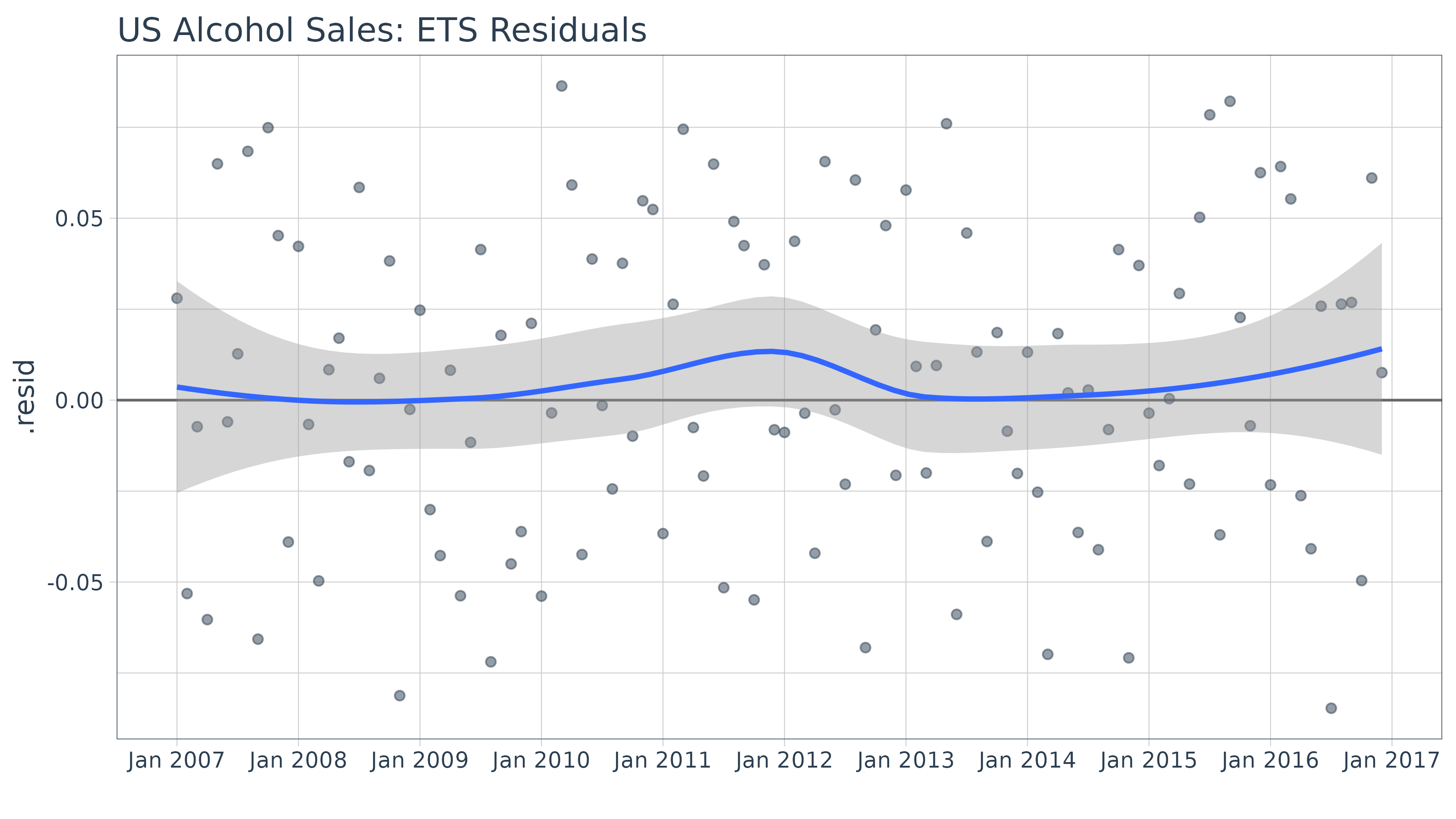

sw_tidy_decomp

sw_tidy_decomp() returns the decomposition of the ETS model.

decomp_fit_ets <- sw_tidy_decomp(fit_ets)
decomp_fit_ets

## # A tibble: 121 × 5
##    index     observed level slope season
##    <yearmon>    <dbl> <dbl> <dbl>  <dbl>
##  1 Dec 2006        NA 8389.  38.9  1.17 
##  2 Jan 2007      6627 8464.  42.0  0.765
##  3 Feb 2007      6743 8433.  32.6  0.837
##  4 Mar 2007      8195 8455.  30.5  0.975
##  5 Apr 2007      7828 8404.  20.4  0.982
##  6 May 2007      9570 8510.  29.6  1.07 
##  7 Jun 2007      9484 8531.  27.8  1.12 
##  8 Jul 2007      8608 8575.  29.0  0.993
##  9 Aug 2007      9543 8697.  38.7  1.04 
## 10 Sep 2007      8123 8643.  27.2  0.995
## # ℹ 111 more rows

We can review the decomposition using ggplot2 as well. The data will need to be manipulated slightly for the facet visualization. The gather() function from the tidyr package is used to reshape the data into a long format data frame with column names “key” and “value” indicating all columns except for index are to be reshaped. The “key” column is then mutated using mutate() to a factor which preserves the order of the keys so “observed” comes first when plotting.

decomp_fit_ets %>%
    tidyr::gather(key = key, value = value, -index) %>%
    dplyr::mutate(key = as.factor(key)) %>%
    ggplot(aes(x = index, y = value, group = key)) +
    geom_line(color = palette_light()[[2]]) +
    geom_ma(ma_fun = SMA, n = 12, size = 1) +
    facet_wrap(~ key, scales = "free_y") +
    scale_x_yearmon(n = 10) +
    labs(title = "US Alcohol Sales: ETS Decomposition", x = "") + 
    theme_tq() +
    theme(axis.text.x = element_text(angle = 45, hjust = 1))

## Warning: Using the `size` aesthetic in this geom was deprecated in ggplot2 3.4.0.
## ℹ Please use `linewidth` in the `default_aes` field and elsewhere instead.
## This warning is displayed once every 8 hours.
## Call `lifecycle::last_lifecycle_warnings()` to see where this warning was
## generated.

## Warning: Removed 1 row containing missing values (`geom_line()`).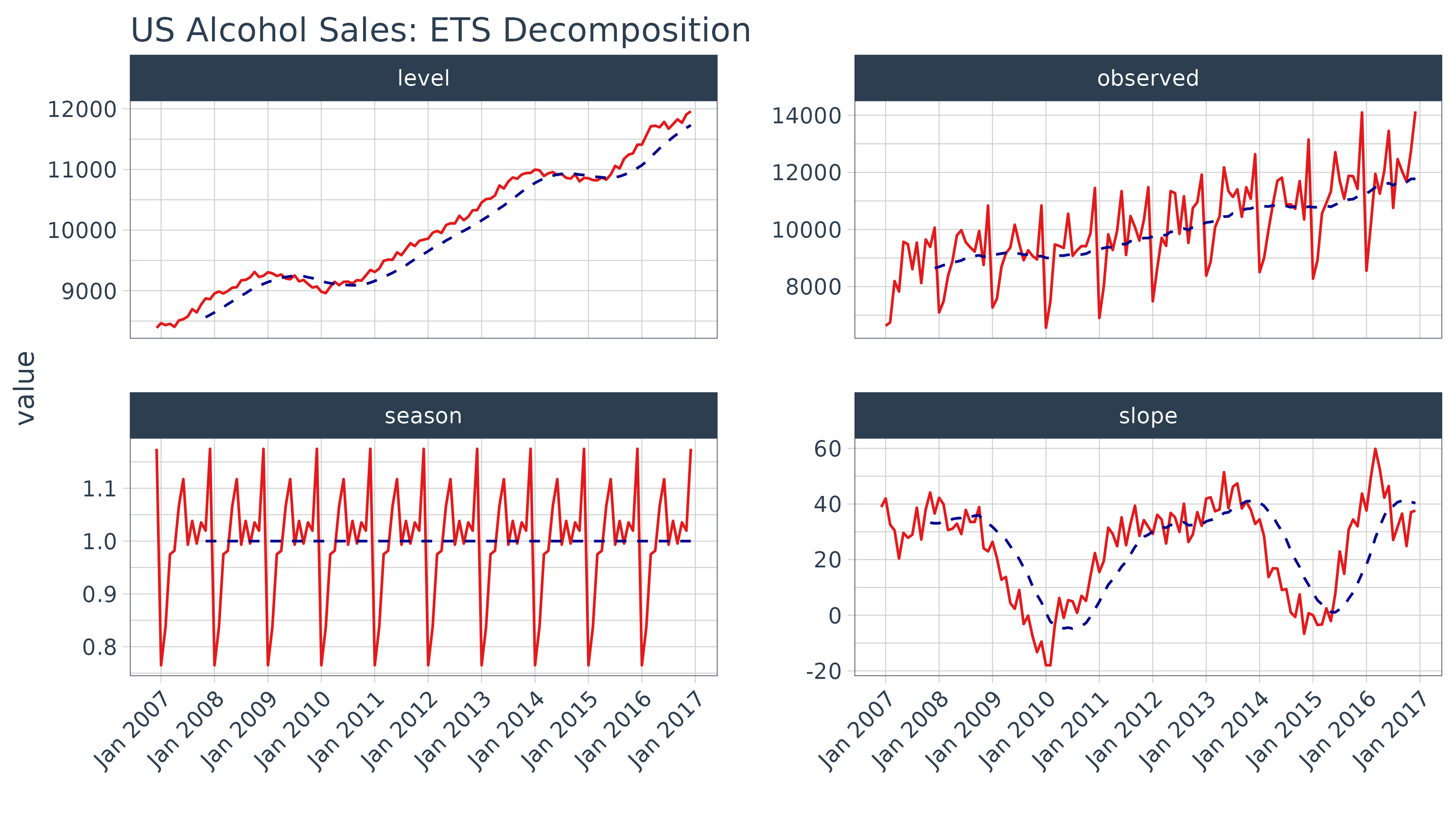

Under normal circumstances it would make sense to refine the model at this point. However, in the interest of showing capabilities (rather than how to forecast) we move onto forecasting the model. For more information on how to forecast, please refer to the online book “Forecasting: principles and practices”.

Step 3: Forecasting the model

Next we forecast the ETS model using the forecast() function. The returned forecast object isn’t in a “tidy” format (i.e. data frame). This is where the sw_sweep() function helps.

fcast_ets <- fit_ets %>%
    forecast(h = 12)

Step 4: Tidy the forecast object

We’ll use the sw_sweep() function to coerce a forecast into a “tidy” data frame. The sw_sweep() function then coerces the forecast object into a tibble that can be sent to ggplot for visualization. Let’s inspect the result.

sw_sweep(fcast_ets, fitted = TRUE)

## # A tibble: 252 × 7
##    index     key    price lo.80 lo.95 hi.80 hi.95
##    <yearmon> <chr>  <dbl> <dbl> <dbl> <dbl> <dbl>
##  1 Jan 2007  actual  6627    NA    NA    NA    NA
##  2 Feb 2007  actual  6743    NA    NA    NA    NA
##  3 Mar 2007  actual  8195    NA    NA    NA    NA
##  4 Apr 2007  actual  7828    NA    NA    NA    NA
##  5 May 2007  actual  9570    NA    NA    NA    NA
##  6 Jun 2007  actual  9484    NA    NA    NA    NA
##  7 Jul 2007  actual  8608    NA    NA    NA    NA
##  8 Aug 2007  actual  9543    NA    NA    NA    NA
##  9 Sep 2007  actual  8123    NA    NA    NA    NA
## 10 Oct 2007  actual  9649    NA    NA    NA    NA
## # ℹ 242 more rows

The tibble returned contains “index”, “key” and “value” (or in this case “price”) columns in a long or “tidy” format that is ideal for visualization with ggplot2. The “index” is in a regularized format (in this case yearmon) because the forecast package uses ts objects. We’ll see how we can get back to the original irregularized format (in this case date) later. The “key” and “price” columns contains three groups of key-value pairs:

actual: the actual values from the original data
fitted: the model values returned from the ets() function (excluded by default)
forecast: the predicted values from the forecast() function

The sw_sweep() function contains an argument fitted = FALSE by default meaning that the model “fitted” values are not returned. We can toggle this on if desired. The remaining columns are the forecast confidence intervals (typically 80 and 95, but this can be changed with forecast(level = c(80, 95))). These columns are setup in a wide format to enable using the geom_ribbon().

Let’s visualize the forecast with ggplot2. We’ll use a combination of geom_line() and geom_ribbon(). The fitted values are toggled off by default to reduce the complexity of the plot, but these can be added if desired. Note that because we are using a regular time index of the yearmon class, we need to add scale_x_yearmon().

sw_sweep(fcast_ets) %>%
    ggplot(aes(x = index, y = price, color = key)) +
    geom_ribbon(aes(ymin = lo.95, ymax = hi.95), 
                fill = "#D5DBFF", color = NA, linewidth = 0) +
    geom_ribbon(aes(ymin = lo.80, ymax = hi.80, fill = key), 
                fill = "#596DD5", color = NA, linewidth = 0, alpha = 0.8) +
    geom_line(linewidth = 1) +
    labs(title = "US Alcohol Sales, ETS Model Forecast", x = "", y = "Millions",
         subtitle = "Regular Time Index") +
    scale_y_continuous(labels = scales::label_dollar()) +
    scale_x_yearmon(n = 12, format = "%Y") +
    scale_color_tq() +
    scale_fill_tq() +
    theme_tq()

Because the ts object was created with the tk_ts() function, it contained a timetk index that was carried with it throughout the forecasting workflow. As a result, we can use the timetk_idx argument, which maps the original irregular index (dates) and a generated future index to the regularized time series (yearmon). This results in the ability to return an index of date and datetime, which is not currently possible with the forecast objects. Notice that the index is returned as date class.

sw_sweep(fcast_ets, timetk_idx = TRUE) %>%
    head()

## Warning in .check_tzones(e1, e2): 'tzone' attributes are inconsistent

## # A tibble: 6 × 7
##   index      key    price lo.80 lo.95 hi.80 hi.95
##   <date>     <chr>  <dbl> <dbl> <dbl> <dbl> <dbl>
## 1 2007-01-01 actual  6627    NA    NA    NA    NA
## 2 2007-02-01 actual  6743    NA    NA    NA    NA
## 3 2007-03-01 actual  8195    NA    NA    NA    NA
## 4 2007-04-01 actual  7828    NA    NA    NA    NA
## 5 2007-05-01 actual  9570    NA    NA    NA    NA
## 6 2007-06-01 actual  9484    NA    NA    NA    NA

sw_sweep(fcast_ets, timetk_idx = TRUE) %>%
    tail()

## Warning in .check_tzones(e1, e2): 'tzone' attributes are inconsistent

## # A tibble: 6 × 7
##   index      key       price  lo.80  lo.95  hi.80  hi.95
##   <date>     <chr>     <dbl>  <dbl>  <dbl>  <dbl>  <dbl>
## 1 2017-07-01 forecast 12117. 11309. 10882. 12924. 13351.
## 2 2017-08-01 forecast 12697. 11828. 11367. 13566. 14027.
## 3 2017-09-01 forecast 12203. 11343. 10888. 13063. 13518.
## 4 2017-10-01 forecast 12723. 11800. 11311. 13647. 14136.
## 5 2017-11-01 forecast 12559. 11619. 11122. 13499. 13996.
## 6 2017-12-01 forecast 14499. 13380. 12788. 15618. 16211.

We can build the same plot with dates in the x-axis now.

sw_sweep(fcast_ets, timetk_idx = TRUE) %>%
    ggplot(aes(x = index, y = price, color = key)) +
    geom_ribbon(aes(ymin = lo.95, ymax = hi.95), 
                fill = "#D5DBFF", color = NA, linewidth = 0) +
    geom_ribbon(aes(ymin = lo.80, ymax = hi.80, fill = key), 
                fill = "#596DD5", color = NA, linewidth = 0, alpha = 0.8) +
    geom_line(linewidth = 1) +
    labs(title = "US Alcohol Sales, ETS Model Forecast", x = "", y = "Millions", 
         subtitle = "Irregular Time Index") +
    scale_y_continuous(labels = scales::dollar) +
    scale_x_date(date_breaks = "1 year", date_labels = "%Y") +
    scale_color_tq() +
    scale_fill_tq() +
    theme_tq()

## Warning in .check_tzones(e1, e2): 'tzone' attributes are inconsistent

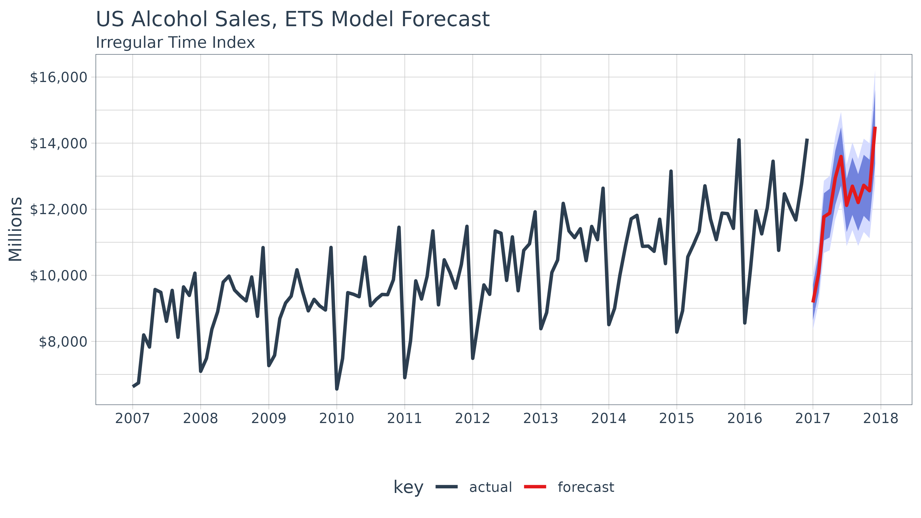
In this example, there is not much benefit to returning an irregular time series. However, when working with frequencies below monthly, the ability to return irregular index values becomes more apparent.

Recap

This was an overview of how various functions within the sweep package can be used to assist in forecast analysis. In the next vignette, we discuss some more powerful concepts including forecasting at scale with grouped time series analysis.

Matt Dancho

2024-01-04

Prerequisites

Forecasting Sales of Beer, Wine, and Distilled Alcohol Beverages

Forecasting Workflow

Step 1: Coerce to a `ts` object class

Step 2: Modeling a time series

sw_tidy

sw_glance

sw_augment

sw_tidy_decomp

Step 3: Forecasting the model

Step 4: Tidy the forecast object

Recap

Introduction to sweep

Matt Dancho

2024-01-04

Prerequisites

Forecasting Sales of Beer, Wine, and Distilled Alcohol Beverages

Forecasting Workflow

Step 1: Coerce to a ts object class

Step 2: Modeling a time series

sw_tidy

sw_glance

sw_augment

sw_tidy_decomp

Step 3: Forecasting the model

Step 4: Tidy the forecast object

Recap

Step 1: Coerce to a `ts` object class